Available now with the Native Planning Engine. Driver-Based Planning in Fabric Plan relies on the Native Planning Engine’s file-based architecture in OneLake and is not supported by the previous planning engine. Turn on the engine at the tenant and workspace levels to start using it.
Your sales team revises its shipment forecast ahead of the holiday season. Operations expects higher delivery volumes, and finance needs to understand the cost impact.
The business relationship is straightforward: more shipments mean more delivery expense. Updating the plan should be just as straightforward.
In a spreadsheet, someone needs to connect the right cells, copy formulas across periods, check references, and maintain separate assumptions for different regions. In a planning application, a similar change may require additional model configuration before planners can use it. As the plan grows, these connections take more effort to maintain.
Driver-Based Planning lets you configure a relationship directly in your Fabric Plan sheet. Choose the row and measure you want to calculate, select the row and measure that will drive it, and define the operation. Keep the assumption visible in the grid, where planners can review and change it.
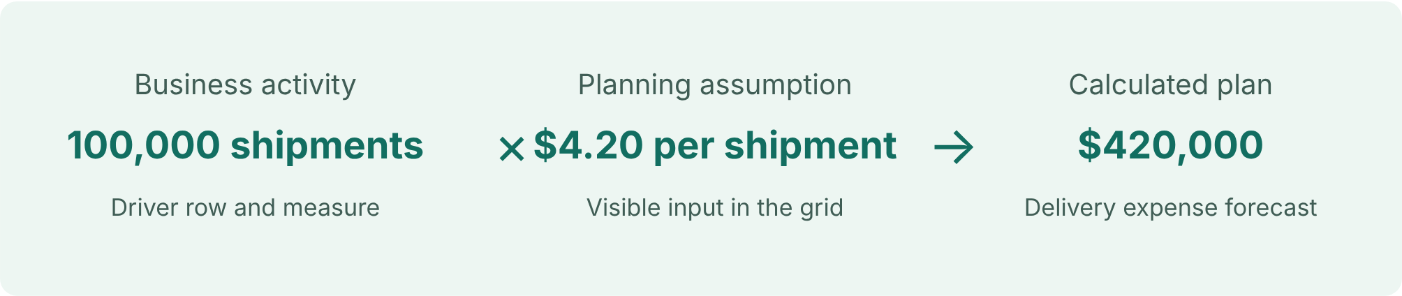
A logistics company is preparing its fourth-quarter operating plan. Delivery expense depends on forecast shipment volumes and an expected cost of $4.20 per shipment.
| Planning item | October | November | December |
|---|---|---|---|
| Forecast shipments | 100,000 | 120,000 | 180,000 |
| Cost per shipment | $4.20 | $4.20 | $4.20 |
| Delivery expense | $420,000 | $504,000 | $756,000 |
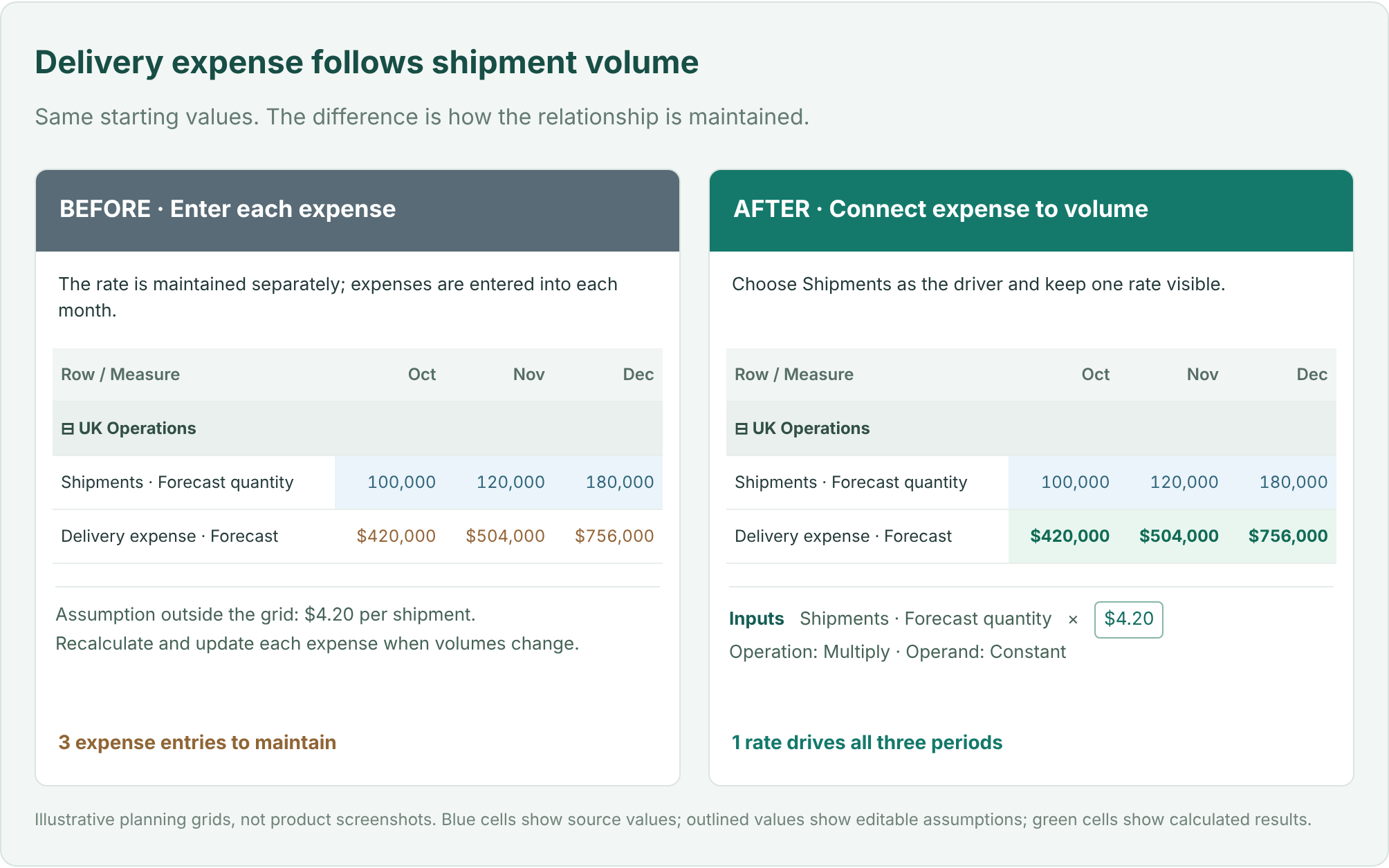
Entering the expense estimates separately creates unnecessary work whenever volumes change. Connecting them to the shipment forecast keeps the business assumption consistent.
If November’s volume increases from 120,000 to 140,000 shipments, delivery expense becomes $588,000 at the same rate. Finance can focus on the impact of that change instead of rebuilding the calculation.
A row can contain several measures, such as quantity, price, revenue, and forecast. Selecting a row alone does not identify which value should be calculated. Driver-Based Planning makes the destination and source explicit.
| Configuration | Logistics example |
|---|---|
| Destination row | UK Operations → Delivery expense |
| Destination measure | Forecast |
| Driver row | UK Operations → Shipments |
| Driver measure | Forecast quantity |
The measures can differ: a quantity measure can drive an expense measure. The destination must be an eligible Data Input target; the driver can use an available source measure, including a native measure.
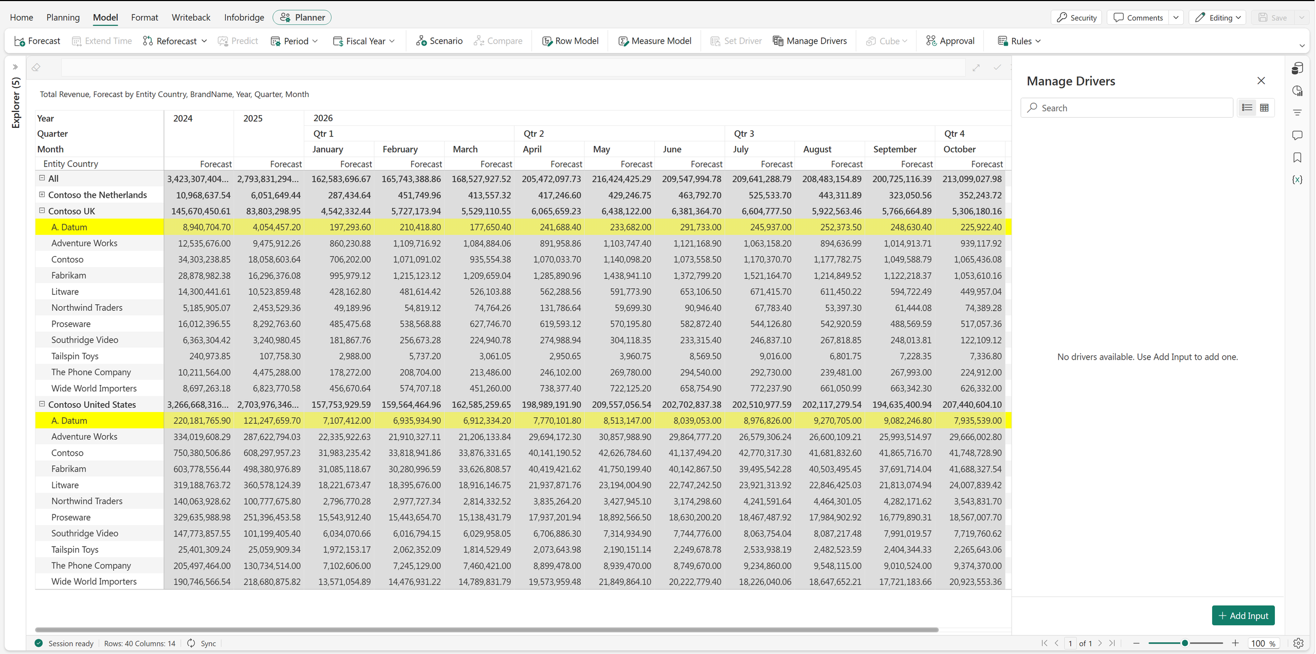
Open Model → Manage Drivers → Add Input and select the destination row from the hierarchy.
All of these settings are in the Set Driver panel.
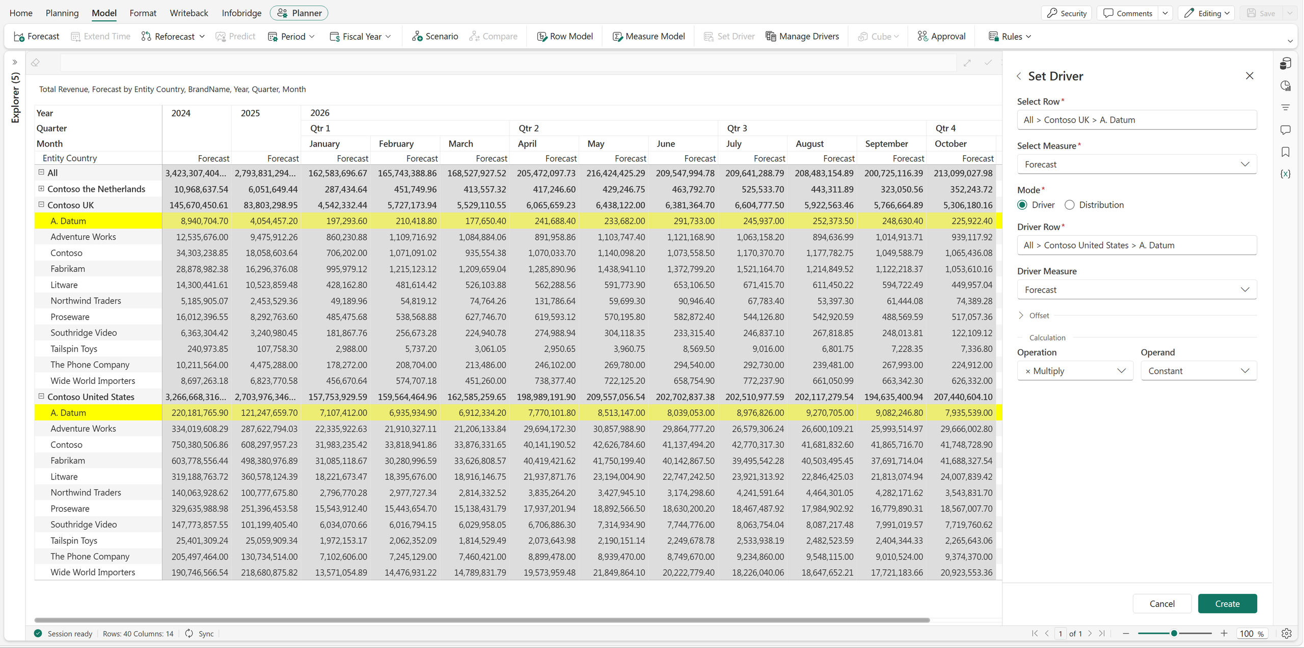
With Constant, one visible assumption applies across the periods governed by the rule. Planners can see and adjust the rate without searching through cell formulas.
Delivery rates often rise during peak season. The logistics company expects a November surcharge and a higher December rate. A single constant no longer represents the business.
Change Operand to Value by Month. Fabric Plan displays input boxes across the periods. Enter the appropriate delivery rate for each month.
| Planning item | October | November | December |
|---|---|---|---|
| Forecast shipments | 100,000 | 120,000 | 180,000 |
| Monthly delivery rate | $4.20 | $4.60 | $4.80 |
| Delivery expense | $420,000 | $552,000 | $864,000 |
The quarter’s expense is now $1,836,000, compared with $1,680,000 at a constant $4.20 rate. The additional $156,000 has a clear explanation: the volumes are unchanged, but the November and December rates are higher.
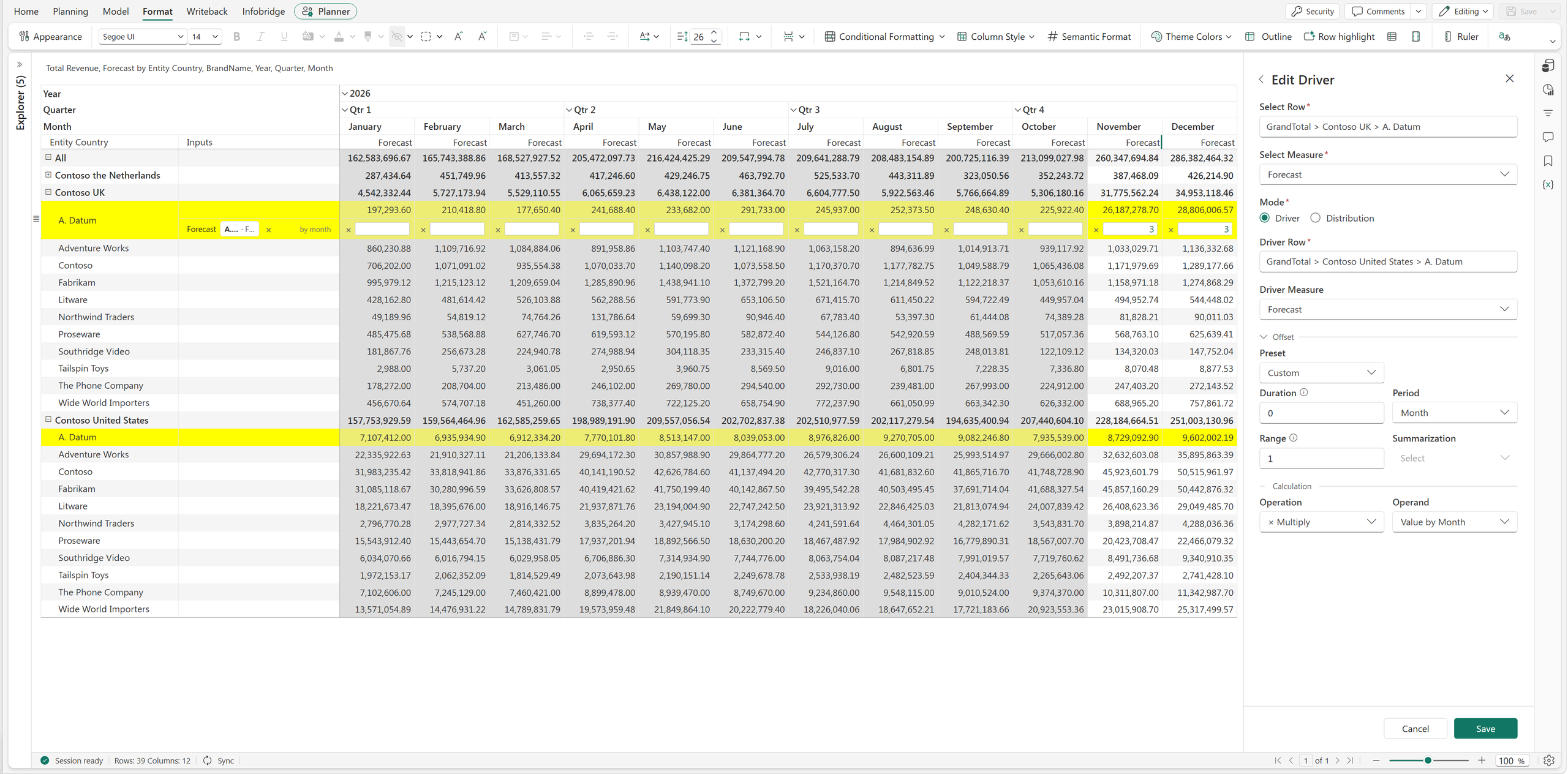
This is useful for seasonal costs, scheduled price changes, and productivity assumptions. The relationship stays consistent while the inputs reflect the business calendar.
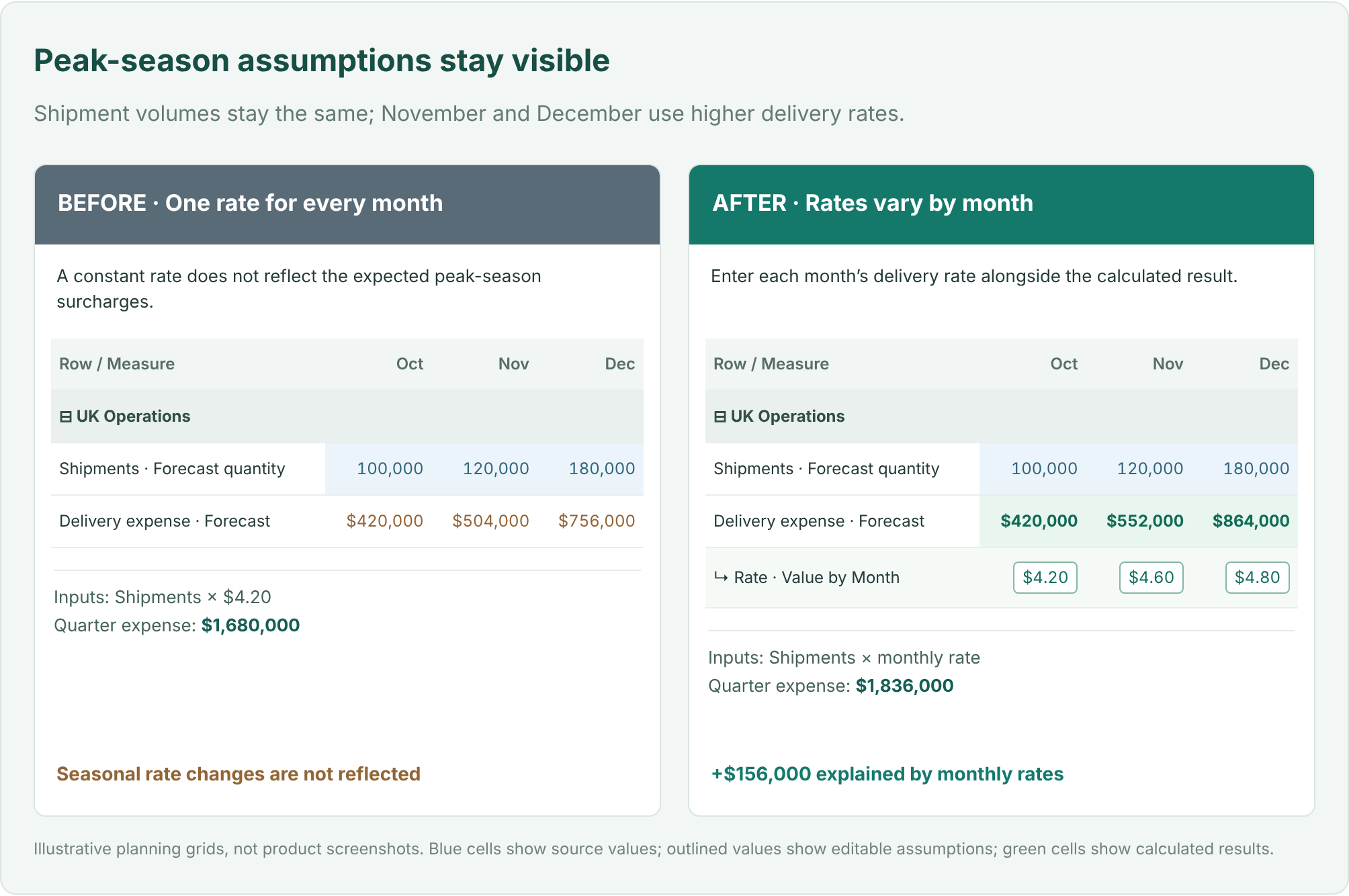
Driver mode supports five operations. Each rule applies one operation to the selected driver value, using a constant or a period-specific operand.
| Operation | Business example | Result |
|---|---|---|
| Multiply | Shipments × cost per shipment | 100,000 × $4.20 = $420,000 |
| Percentage | Revenue at a commission rate | $2,000,000 at 3% = $60,000 |
| Divide | Labor hours ÷ hours per FTE | 16,000 ÷ 160 = 100 FTE |
| Add | Baseline demand + extra units | 100,000 + 5,000 = 105,000 |
| Subtract | Gross demand − canceled units | 100,000 − 2,000 = 98,000 |
Taking a percentage and increasing a value by a percentage are different questions. A 3% commission is 3% of revenue. A 3% uplift can be expressed by multiplying the baseline by 1.03.
Not every plan should follow the current period’s value. You may want to carry forward an earlier month, smooth recent volatility with an average, or use a total across a historical window.
Open Offset to choose a preset.
| Preset | What it does | Input |
|---|---|---|
| Prior Period | References an earlier period | Go back |
| Rolling Average | Averages values across a window | Window |
| Rolling Total | Totals values across a window | Window |
| Custom | Sets the reference window explicitly | Duration, Period, Range, Summarization |
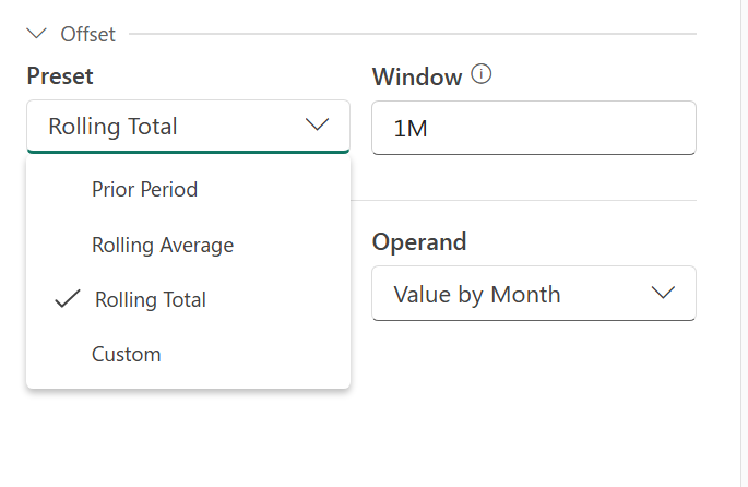
For Prior Period, enter 1M to go back one month, 1Q for one quarter, or 1Y for one year. Rolling Average and Rolling Total use a Window input to specify the period span.
Suppose finance wants November’s baseline delivery expense to reflect the average shipment volume from July through October.
| Historical month | Shipments |
|---|---|
| July | 80,000 |
| August | 90,000 |
| September | 110,000 |
| October | 100,000 |
| Four-month average | 95,000 |
Select Custom and configure Duration = 1, Period = Month, Range = 4, and Summarization = Average. Keep the operation as Multiply and enter a constant of 4.20.
For November, Duration moves the reference point back to October. Range includes four consecutive months ending there: July, August, September, and October. The average is 95,000 shipments, so the baseline expense is $399,000.
Duration determines how far back to look. Range determines how many periods to include. Summarization combines those values using Average, Sum, Lowest, or Highest. The selected historical value then feeds the calculation.
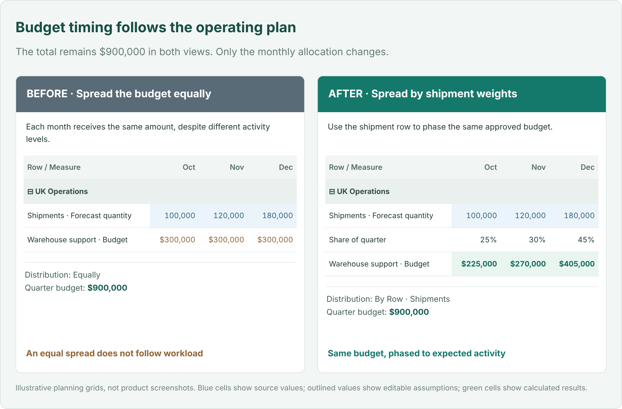
The logistics company has approved a $900,000 quarterly warehouse support budget. Finance wants to phase that amount according to expected shipment activity rather than divide it equally.
| Planning item | October | November | December | Total |
|---|---|---|---|---|
| Forecast shipments | 100,000 | 120,000 | 180,000 | 400,000 |
| Share of quarter | 25% | 30% | 45% | 100% |
| Support budget | $225,000 | $270,000 | $405,000 | $900,000 |
Choose the destination row and measure, then switch Mode to Distribution. Choose By Row and select the reference that supplies the shipment weights. Enter the amount to distribute across the relevant periods.
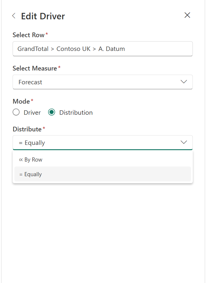
With Equally, the budget would be $300,000 in each month. With By Row, December receives $405,000 because it represents 45% of the quarter’s shipments. The total remains $900,000; the timing reflects the activity it supports.
Offsets also work with the reference values used for distribution weights. You can use an earlier activity pattern when that is a better basis for phasing the budget.
Driver mode calculates a value from a business relationship. Distribution mode spreads an amount across periods.
When the source, operation, and assumption are visible together, it becomes easier to explain a change. Operations can challenge the cost per shipment. Finance can identify which months include a surcharge. Regional managers can see how the budget follows expected activity.
Driver-Based Planning works with both Row Model and Measure Model sheets. Where a row has multiple eligible Data Input measures, each can have its own independent driver configuration.
For a driver-governed result, update the driving value or its assumption. Directly typing over that result does not reverse-solve the driver. This keeps the relationship explicit.
Start with one relationship your team already understands: delivery expense driven by shipments, commissions driven by revenue, or labor requirements driven by workload. Select the destination, choose its driver, and enter the assumption. Then change the source or rate and review the resulting plan.
Spend less time maintaining the connections between numbers, and more time deciding whether the assumptions behind them are right.
Feature details reflect Fabric Plan at the time of writing.