Available now for all Plan items. Anchoring Measures does not require the Native Planning Engine; it works with both the Native Planning Engine and the previous planning engine.
A product’s unit price belongs beside the product. A regional assumption belongs where the regional team maintains it. An executive profitability metric belongs in the summary where leaders review it.
But add those measures to a hierarchical grid, and they can appear everywhere: at region totals, category subtotals, individual SKUs, and every expanded period. The grid treats them alike even though they serve different business purposes.
Anchoring Measures in Fabric Plan lets you choose the row and column levels where each measure belongs. It works with Power BI Measures, input measures created in the plan, and formula measures created in the plan. For input measures, the anchor also defines where users can enter values directly.
You can build one view that shows product details, business assumptions, and executive results at their appropriate levels, with fewer repeated measures to navigate.
Imagine a retailer planning across Region → Category → SKU, with Year → Quarter → Month on columns. The plan includes quantity, unit price, standard unit cost, price uplift, revenue, and EBITDA margin.
Those measures answer different questions. A planner needs quantity at SKU and month. A pricing team maintains an annual uplift by region. Leadership reviews quarterly EBITDA margin by region. A price displayed at the regional subtotal may be technically calculated by the model, but it is not the product price the planner needs.
Without control over placement, teams often accept a cluttered grid, build separate summary and detail reports, or maintain assumptions in a separate spreadsheet block connected to the plan by formulas. Users must remember which repeated values are meaningful and which cells they should update.
Anchoring makes that intent part of the grid configuration. Here are three realistic ways it helps.
A retailer sells two products with centrally maintained prices and standard costs:
| Product SKU | List price per unit | Standard cost per unit |
|---|---|---|
| Travel Mug TM100 | $24 | $9 |
| Water Bottle WB200 | $32 | $12 |
In this example, each SKU’s list price and standard cost are the same across regions. These are Power BI Measures from the Power BI semantic model.
When the measures repeat throughout the hierarchy, the grid also presents them at Category and Region subtotals. Whether the underlying measure returns an average, another aggregate, or a blank, that placement distracts from the intended question: What is the price or cost of this SKU? A regional subtotal is not another product with its own list price.
Teams may work around this with a separate product reference report or special display logic in their measures. That adds maintenance just to control where a number appears.
Anchor List Price and Standard Unit Cost to the SKU level. Users see those measures at product detail, while Region and Category subtotals focus on totals such as quantity, revenue, and gross profit. Hide the non-anchored instances to remove those price and cost measures from the subtotal levels.
The SKU’s $24 price still comes from the Power BI measure. Anchoring controls its placement; it does not force prices to be identical across regions or alter the DAX calculation. The shared regional price is already a rule of this example’s semantic model.
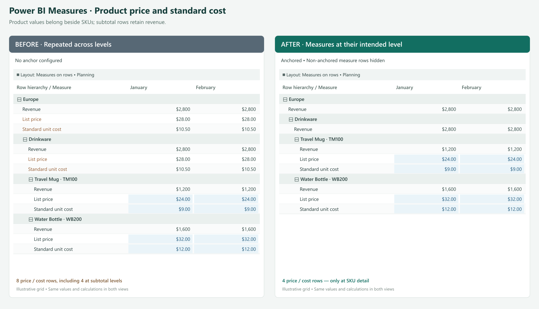
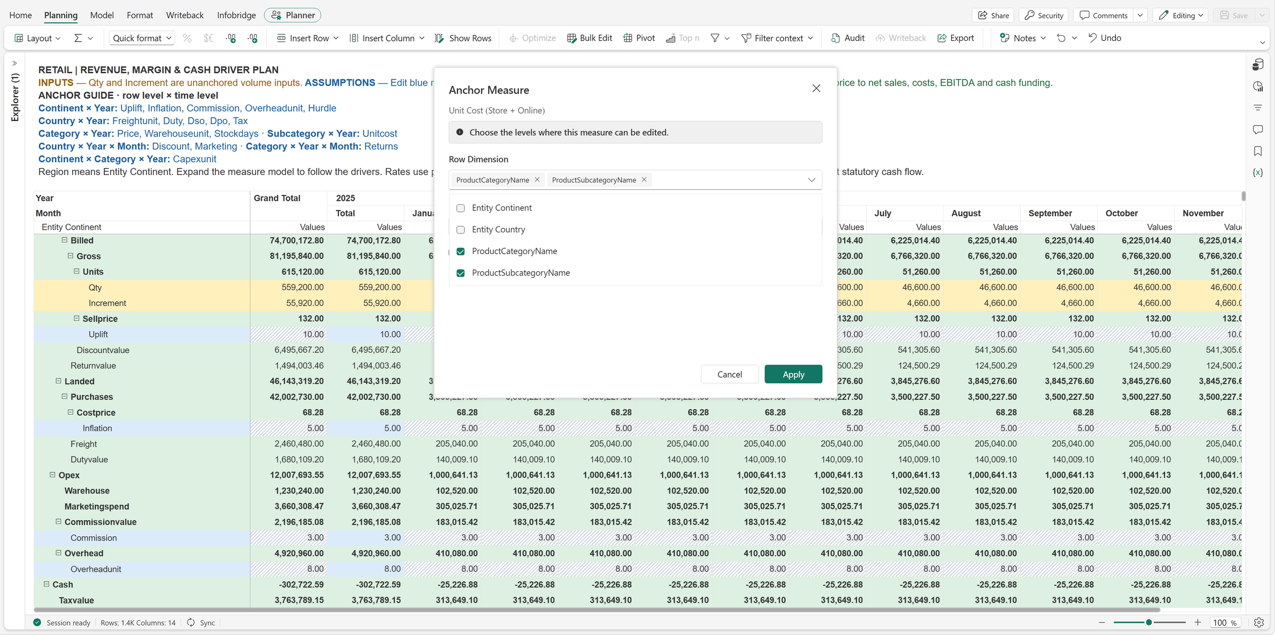
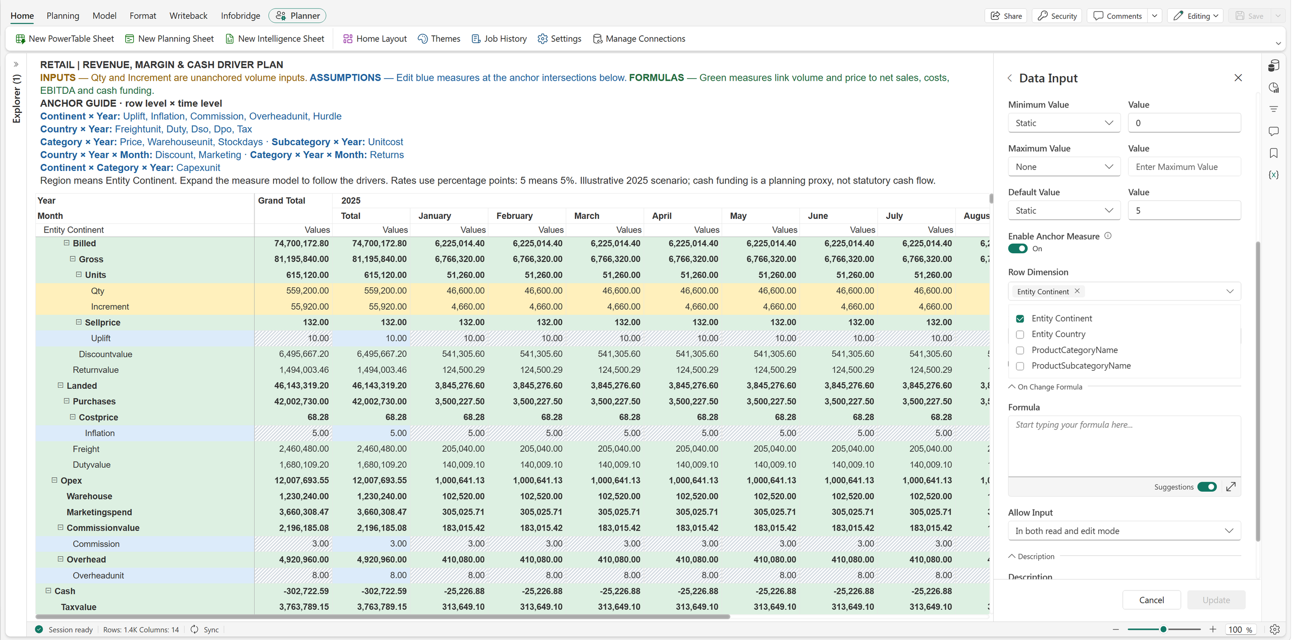
Open Manage Rows (Show Rows on the ribbon) or Manage Columns, locate the Power BI Measure, and click its anchor icon. In Anchor Measure, select the SKU dimension under Row Dimension, then apply the settings. Configure non-anchored instances to be hidden for the product-detail presentation.
The same approach is useful for measures such as standard weight per unit or price per pack when their meaningful reporting level is an individual product.
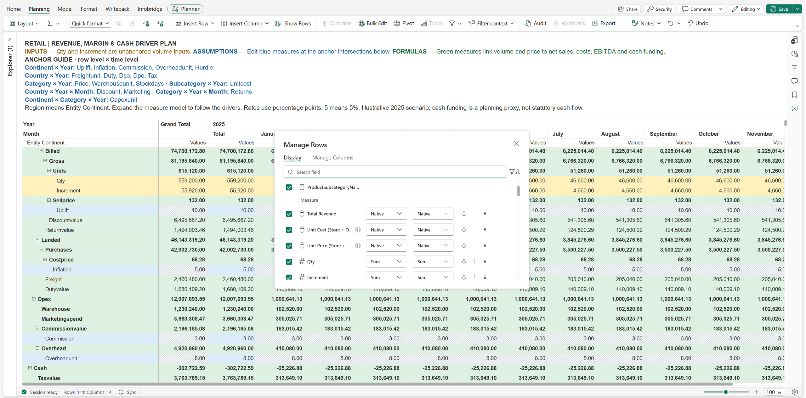
A pricing team agrees on an annual price uplift of 5% for Europe and 3% for North America. The sales plan contains hundreds of SKUs and twelve months of detail.
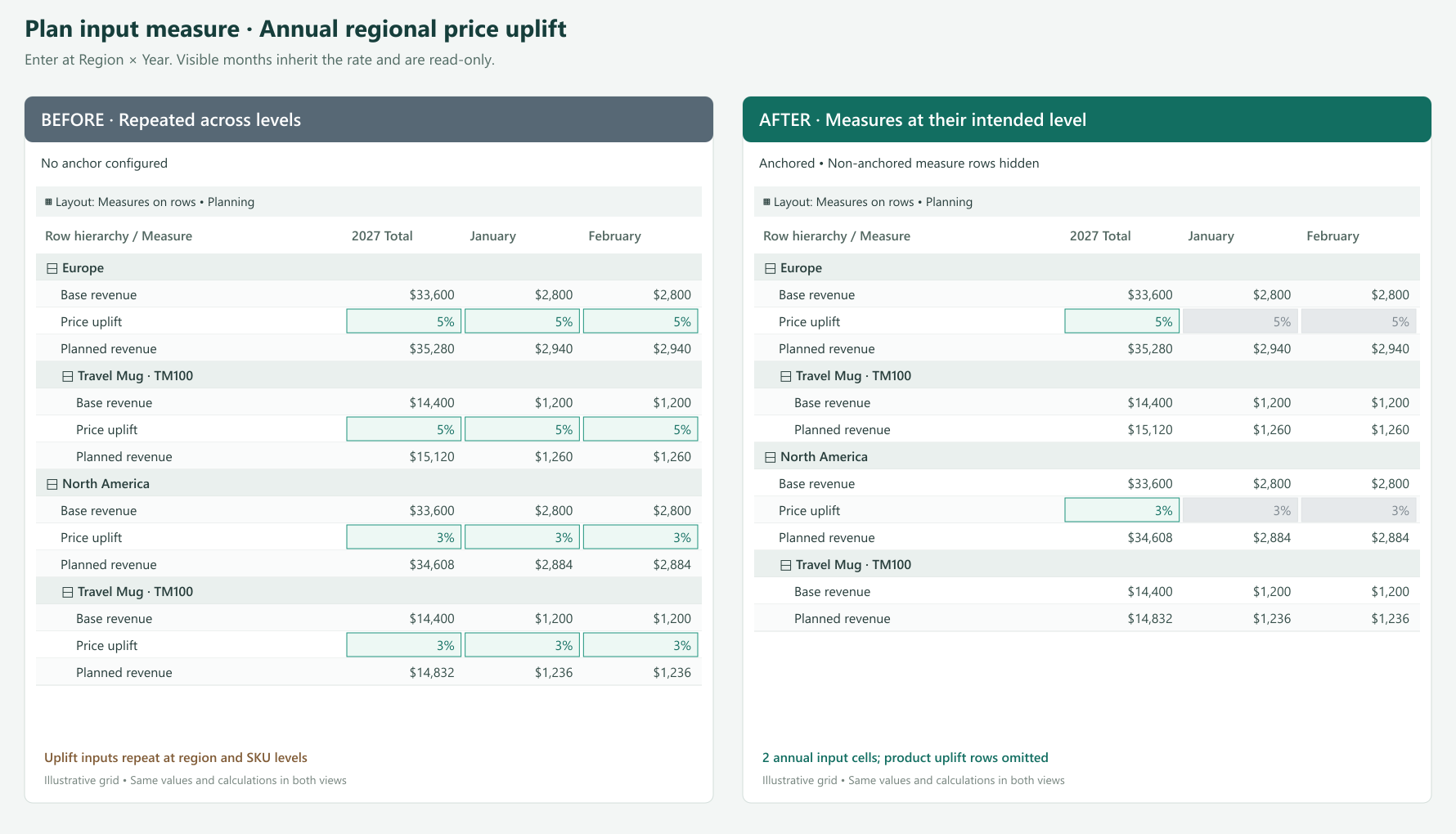
If the uplift is available for direct entry throughout the detail, users have many places to maintain a decision made once per region and year. They may copy the rate across cells or maintain a separate assumptions block above the plan. It becomes harder to tell whether a different value is intentional or an accidental override.
Anchor the Price Uplift input measure to Region × Year. Europe has one annual input point for its 5% assumption; North America has another for 3%. Users enter the values at the corresponding year subtotal.
With the existing distribution configured to repeat the rate, eligible detail receives the regional assumption. A product with a base price of $24 therefore has a planned price of $25.20 in Europe and $24.72 in North America, using:
Planned price = Base price × (1 + Price uplift)
The formula and distribution produce those values. The anchor makes the location for maintaining the assumption explicit. Monthly instances that remain visible are read-only; they are not separate places to override the annual policy.
An annual assumption belongs in the annual subtotal, not January. A quarterly assumption belongs in the quarter subtotal.
| Planning decision | Anchor | What users maintain |
|---|---|---|
| Annual salary increase | Year only | One annual policy shared across the employee plan |
| Regional benefit rate | Region × Year | One annual rate per region, such as 22% or 26% |
| Seasonal demand uplift | Year × Quarter only | One quarterly assumption shared across products and regions |
| Monthly promotion | Country × Year × Month | A discount assumption that varies by country and month |
| Inventory policy | Product category × Year | Annual target stock days for each category |
Neither row nor column selection is individually mandatory. With anchoring enabled, select at least one dimension overall. A time-only seasonal factor can leave Row Dimension empty. A factor that varies only by region can leave Column Dimension empty.
A regional management view includes Revenue, EBITDA, and EBITDA Margin. Users can expand the same grid to inspect categories and SKUs, but leadership wants profitability measures at the regional quarterly summary.
Showing EBITDA and EBITDA Margin beneath every SKU makes operational detail harder to scan. It can also encourage readers to interpret product-level profitability when some operating expenses are managed at a broader level. Teams may maintain a separate executive report simply to keep those measures out of the detail view.
Anchor the plan’s formula measures EBITDA and EBITDA Margin to Region × Year × Quarter. If Region is the top row level, those measures appear at the top business summary level for each region. SKU detail can focus on quantity, price, and revenue.
For example, Europe has quarterly revenue of $2.4 million and EBITDA of $360,000. Its existing formula calculates:
EBITDA Margin = EBITDA ÷ Revenue = 15%
Anchoring places that 15% where leadership reviews the result. It does not average displayed SKU percentages or change how the formula evaluates. Hiding detail instances also does not remove the data or dependencies needed to calculate the summary.
Use the same pattern for Profit Margin or Operating Profit at a selected management level. Choose the highest business dimension you want to present, such as Company, Business Unit, or Region, together with the relevant period.
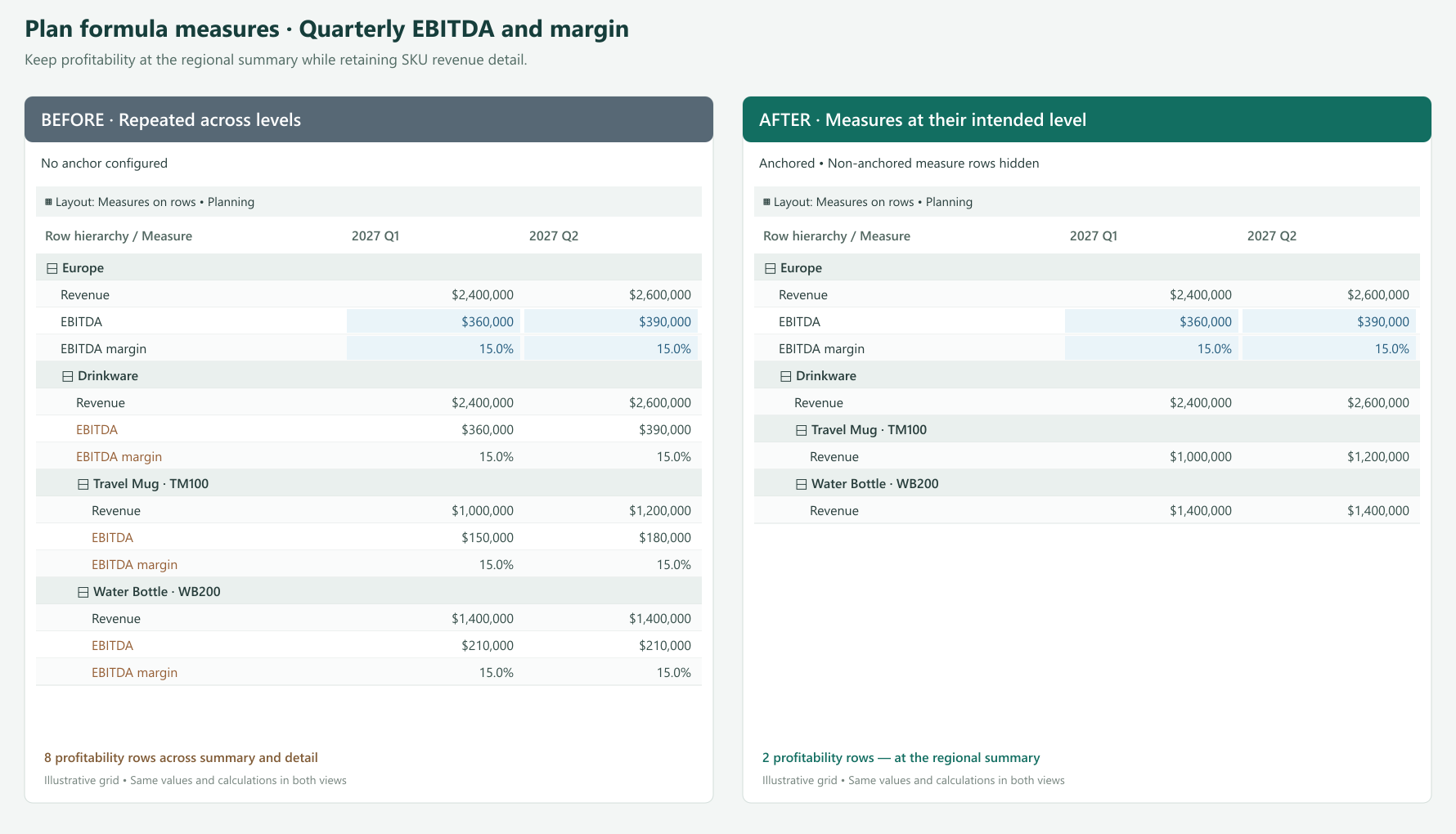
Open the formula measure’s anchor settings through its configuration or the anchor action in Manage Rows / Manage Columns. Select Region as the row dimension and Year and Quarter as the column dimensions. Apply the settings and hide non-anchored instances for the summary-focused presentation.
The formula remains calculated and read-only. Anchoring does not make a formula measure or a Power BI Measure directly editable, even when the shared dialog describes where a measure can be edited.
Show non-anchored instances when users need to follow an assumption into the detail; for input measures, these cells remain read-only. Hide them when the repeated measure adds no useful information.
A regional assumption need not have its own input row under every product in a measures-on-rows layout. A quarterly assumption need not add an input measure column beneath every month in a column layout. Hiding removes unnecessary instances where the layout permits while calculations continue to use the underlying values.
Read-only detail can still receive updates through the existing allocation or distribution process from a valid editable anchor. Normal permissions and locking rules continue to apply. Anchoring controls placement and entry locations; aggregation and allocation settings determine how values are distributed and rolled up.
| Measure type | Example | Appropriate placement | User interaction |
|---|---|---|---|
| Power BI Measure | List price or standard unit cost | SKU detail | Read the existing model value |
| Input measure in the plan | Annual regional uplift | Region × Year subtotal | Enter the assumption at the anchor |
| Input measure in the plan | Quarterly seasonality | All rows × Year × Quarter | Maintain one shared period assumption |
| Formula measure in the plan | EBITDA or profit margin | Management summary × reporting period | Review the calculated result |
Start with a measure that appears in too many places. Put it at the level where it is useful, expand the grid, and check how the detail reads. Then apply the same approach to other measures in the plan.
Product facts at product detail. Assumptions where decisions are made. Results where the business reviews them. Anchoring Measures brings those needs together in one planning and reporting view.
Feature details reflect Fabric Plan at the time of writing.
Measure models in Microsoft Fabric Plan turn the measures in your Power BI semantic model into a plan you can forecast, simulate and optimize, without rebuilding them.
Organizations that report on Power BI spend years deciding what their numbers mean. This includes deciding which sales count as revenue, how margin is worked out and who belongs in the headcount. Those decisions are recorded in the semantic model as measures, and every report that reads from the model inherits them. It is the reason two departments looking at the same figure see the same number.
Planning asks something different of those numbers: how they change when people modify the assumptions behind them.
The usual route to a plan is to take the data out to a separate planning platform. Unfortunately, the logic and calculations in those measures do not travel with it. They need to be defined again in the planning model, and the plan and the reports now end up running on two copies of the business logic.
Fabric Plan takes a different approach. It leaves the definitions where they are and extends them forward, which Microsoft sums up as "Extend, Don't Rebuild". A measure model is the most direct way to do this: it works with the measures you already have, whatever they describe, and turns them into a plan that can be forecast, simulated and tested before anyone commits to it.
Know that this is possible only when you plan directly on top of semantic models. If your plan runs in a separate platform, this approach cannot be used.
In Fabric Plan, a measure model starts from the measures on a planning sheet and arranges them into a hierarchy that reads like the business (e.g., a P&L structure). Forecast measures give each actual a counterpart for the periods ahead, and formula measures combine measures into new ones. Scenarios, simulation and optimization then run across the whole structure. A change to one measure moves up through the measures that depend on it and across the rows at the same time, from a single country up to the total.
Let us explore this through an example.
The example that follows shows actuals by country for 2023 to 2025. Revenue, purchase expense and transportation expense are native measures from the semantic model, and profit actual is a formula built on them. Nothing on the sheet is a plan yet.
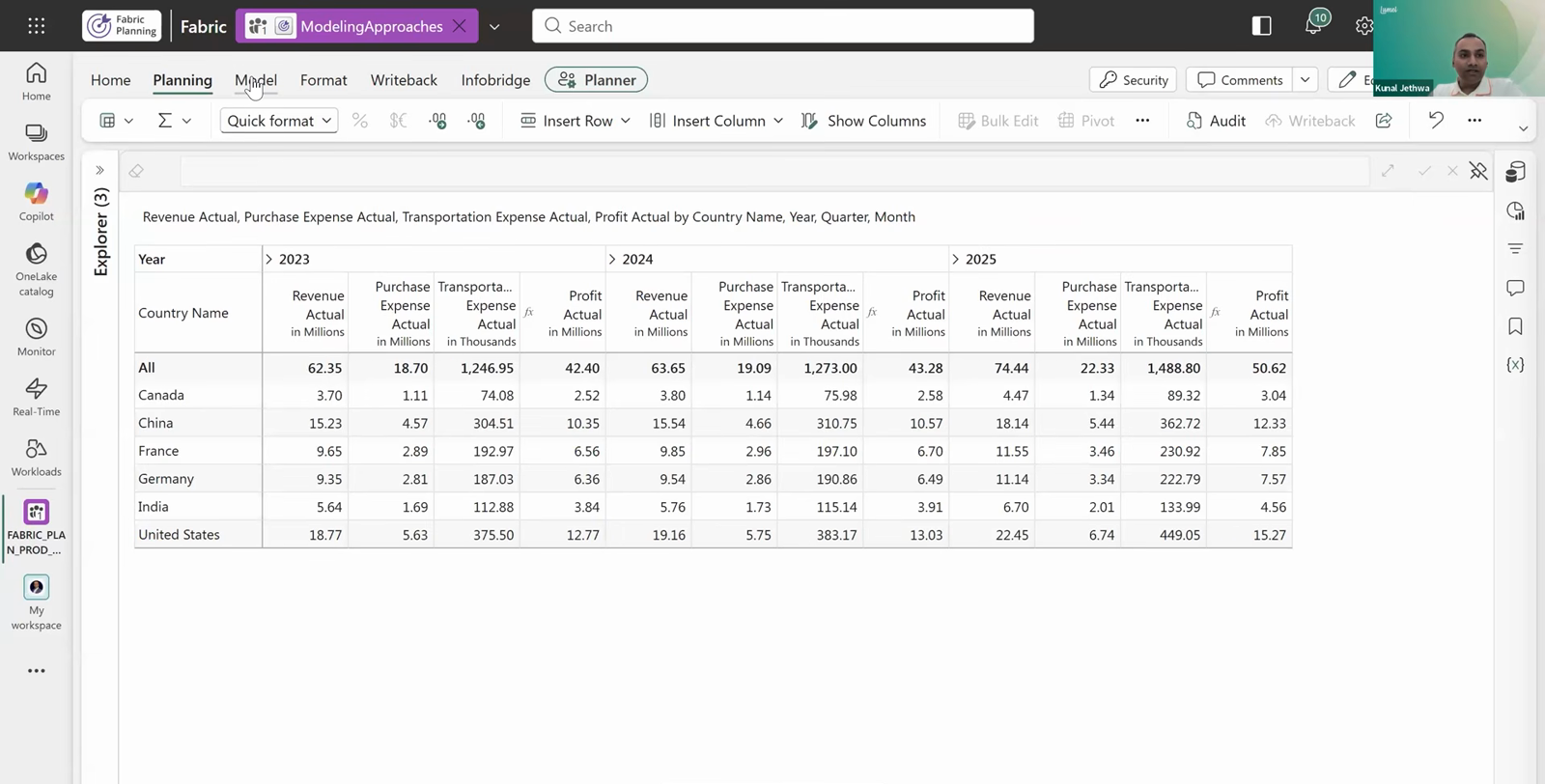
The first step adds a forecast measure for each of the three actuals, covering January to December 2026. For these forecast measures, you may opt to manually enter values (Data Input option), reflect the same values as prior year actual (Link to Measure option) or apply a growth rate of x% (Formula option) over the prior year value.
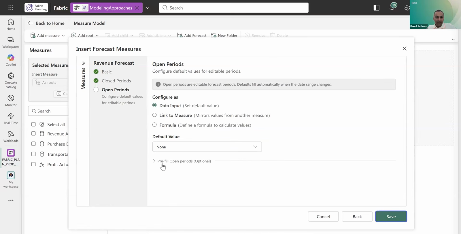
The Profit forecast is a single formula: revenue forecast less purchase and transportation forecast.
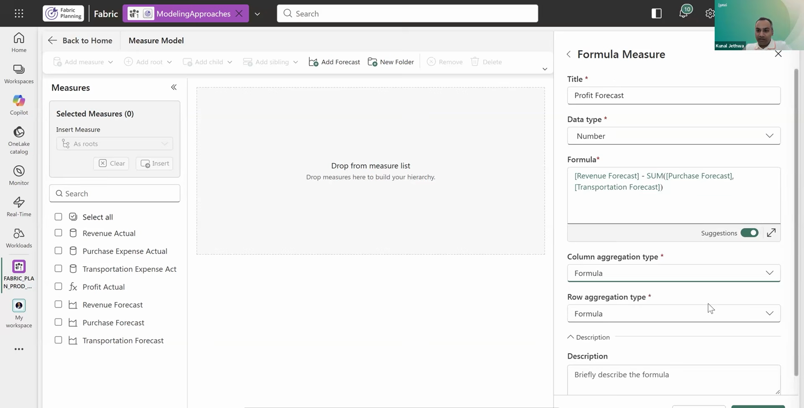
Profit forecast and profit actual then become parents in a tree structure, each with its three constituent measures beneath it. Everything up to this point takes under three minutes to build, and none of the actuals had to be re-created.
To build this yourself, follow the step-by-step tutorial.
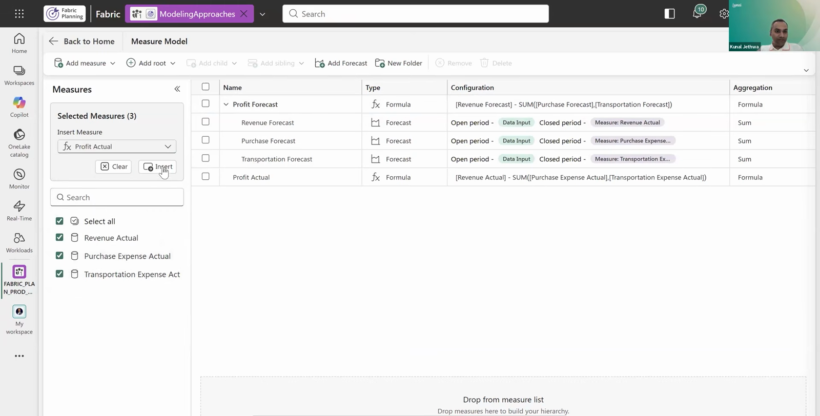
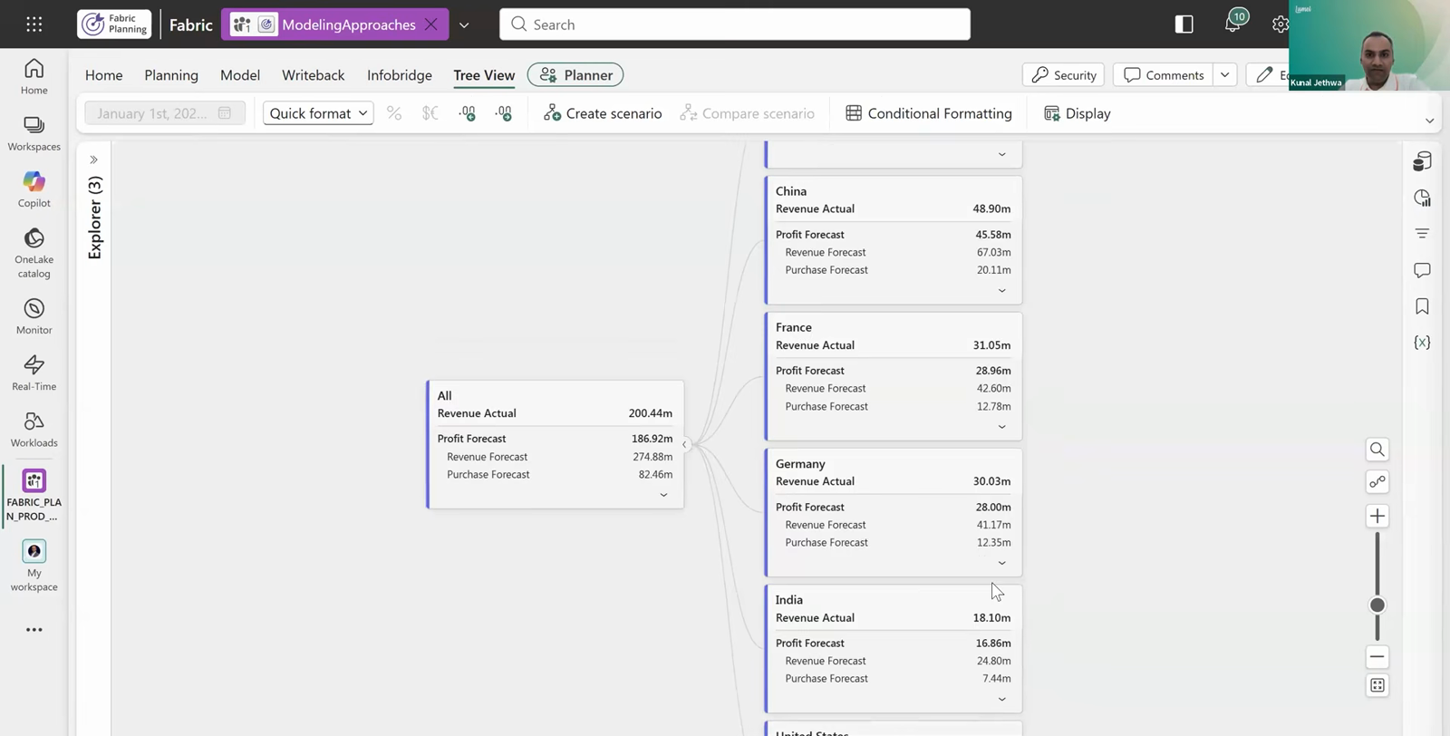
With the model in place, the tree view shows a profit tree for each country, with a visual structure.
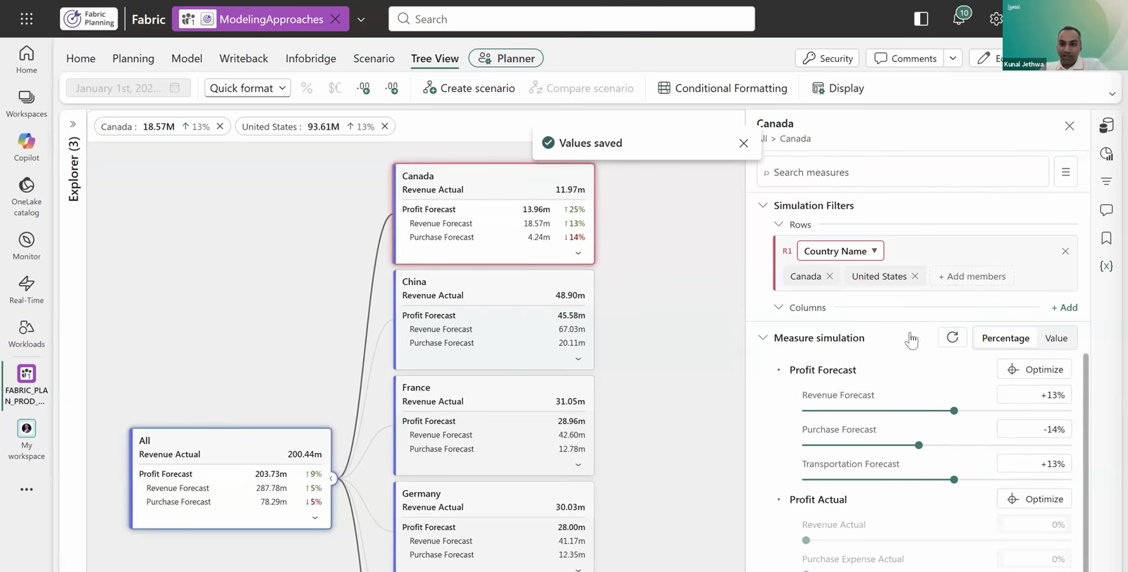
You can run simulations and create scenarios. In our case, revenue and transportation forecast are raised 13% and purchase forecast is cut 14%. This can be applied to both Canada and the United States together. Canada's profit forecast rises 25% as a result, and the overall company profit forecast increases by 9%. These simulations can also be scoped by column, to a quarter, a month or a year.
Simulation answers the question "what happens if these measures change?" The optimizer answers the reverse: what values should the measures take to reach a goal? The Fabric Plan optimizer is a multivariate goal seek. Excel's Goal Seek changes one input to hit one target; the optimizer changes several measures at once and keeps each within the limits you set. In the example it takes four steps.
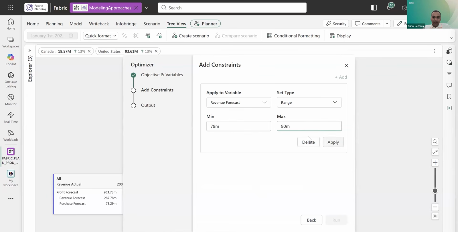
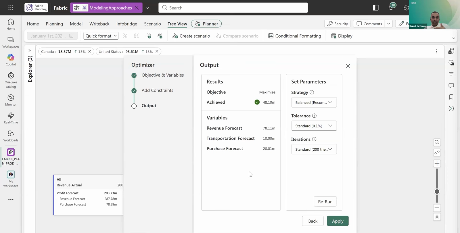
Once the values are applied, Canada's profit forecast and the company total get updated together. The limits in this example were set outside the range of its sample data, so the figures show the mechanics and say nothing about a realistic outcome. The finished scenario can then be compared with others side by side.
The optimizer is not limited to a three-measure tree. It also respects locked values, distribution rules and minimum and maximum rules through multi-level chains of dependent measures.
The example above has three measures. A real plan works with the measures an organization already reports on and runs at a much finer grain, and that is where a measure model is at its strongest. The illustrative product-line P&L below runs from gross sales to operating profit. Eleven of its measures already exist in the semantic model, with their logic written in DAX. The measure model gives each of them a forecast and adds seven formulas for the subtotals.
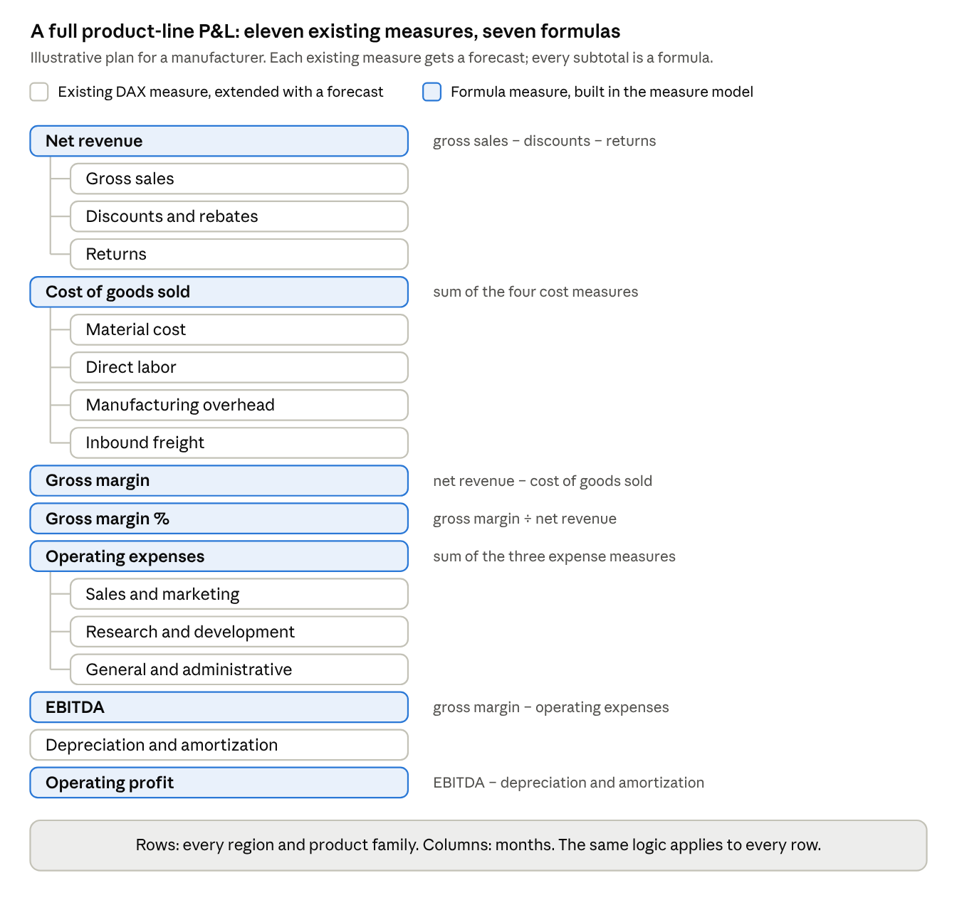
Illustrative product-line P&L · 11 existing measures, 7 formulas
None of the eleven measures is rebuilt. Gross sales may already convert currencies, and material cost may already apply standard costs. That logic stays in the semantic model, and each forecast starts from it. Planners enter forecasts by region and product family, and every subtotal from net revenue to operating profit recalculates. Because a measure model applies the same logic to every row, a new region or product family adds rows to the grid and leaves the model as it is.
Not every plan has this shape. When the logic has to be built line by line in the planning layer, with each line following its own rules, Fabric Plan offers row models in Model Builder. The Planning at Scale blog compares the two.
How quickly a plan goes live is decided mostly by what has to be built before anyone can capture a projection.
With Fabric Plan on a well-governed semantic model, that time-to-market is fast. The data is already in Fabric, the business definitions are already in the measures and row-level security defined on the semantic model applies to the plan without a second setup. What remains is the plan itself: forecasts, the formulas for results and the scenarios to test them. Lumel has seen customers with a strong semantic model go live on headcount planning in under a week.
A standalone planning tool like Anaplan, Pigment or OneStream starts further back. You begin by setting up the master data and bringing transactions from ERP, CRM and HR systems into the planning platform. This setup typically runs twelve weeks or more before any planning logic is rebuilt on top. Implementations of legacy suites such as Oracle Hyperion and SAP BPC typically take six to twelve months to go live.
Watch the full demo of measure models in Fabric Plan: Extend Plans with Measure Models in Microsoft Fabric Planning.