Available now for all Plan items. Consolidation Templates do not require the Native Planning Engine; they work with both the Native Planning Engine and the previous planning engine.
Consolidation Templates work with Row Models, which are what you reach for when your planning logic sits on the rows and different rows need their own logic. You’ll find Row Model in the Model tab of a Planning Sheet, in the Row-based group.

Picture your group finance team in the middle of a quarter close. The group has two organizations, each split into regions, branches and departments, and the departments don’t all report the same things. The sales teams report gross margin, Marketing only has expenses, and Accounts and Finance adds interest, other income and tax on top. The CFO wants to see the whole group first, then each organization, then a single branch, and every total has to tie back to the members underneath it.
The question behind all of this is simple enough: how does each member roll up to the group? The hard part is keeping the answer right every time someone changes the view.
Without a rollup rule on each row, getting there is slow and mostly manual. Someone builds a consolidation layer by hand, copies the formulas across whenever a new member shows up, lays the numbers out again for each audience, and then checks that the totals still add up. The same rework comes back every period, and it gets bigger with each region, division or branch you add.
With Consolidation Templates, you build each statement once as a template with its own structure of rows, and tell every row how it should combine across members. After that you can pivot to whatever level you need and filter to whatever scope you need, and the numbers still add up, because the full model keeps calculating in the background and the pivot is only a view of it. Finance is the worked example in this post, but the same pattern fits any metrics that many people read at different levels.
A group view is only worth having if people trust it and can get it when they need it. Without a rollup rule on each row, both of those depend on a lot of manual effort, and most of that effort lands on the same few people. Here’s what that usually looks like.
Consolidation Templates take that work off your plate. You list your metrics and say how each one rolls up, and the model handles the rest, whichever level you look at, whoever’s asking and however many new members show up.
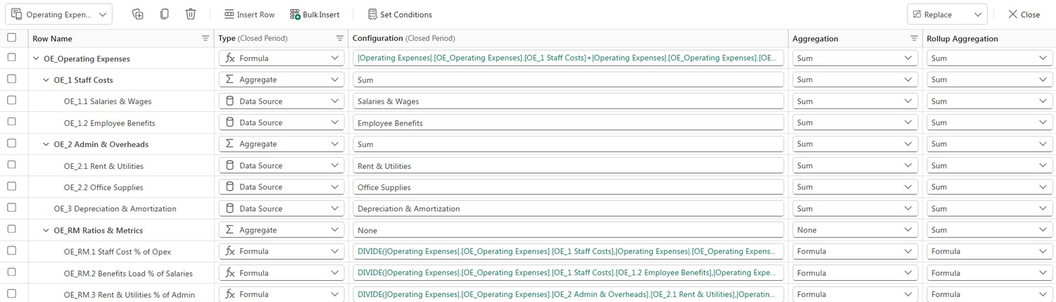
A template isn’t just one row. It’s a whole tree, with a top row, groups underneath it, the inputs at the bottom and a set of ratio rows for the metrics people look at most. The sample model has five of them, and each has a structure of its own. Gross Margin and Operating Expenses are shown in full below.
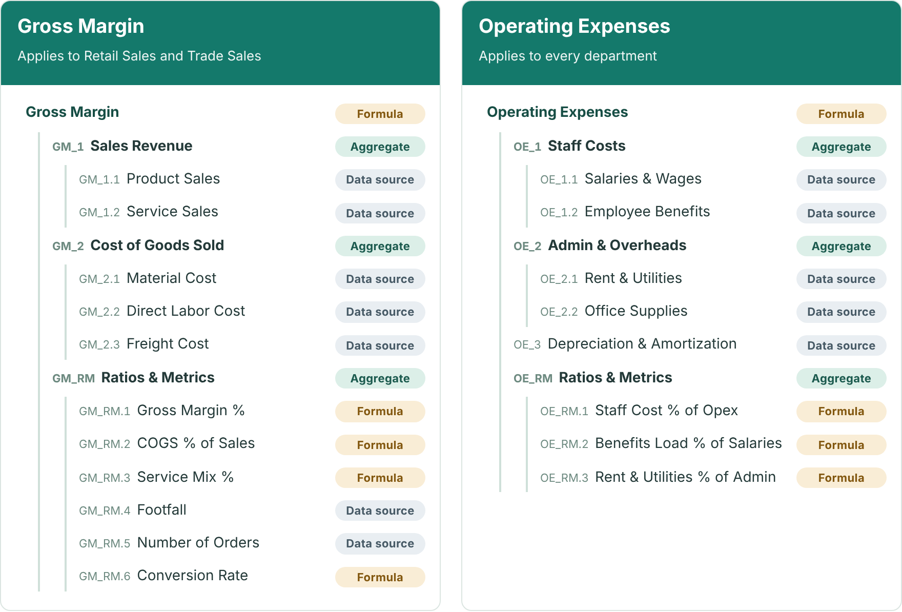
The other three follow the same pattern on a smaller scale, and in the sample model they sit under Accounts and Finance.
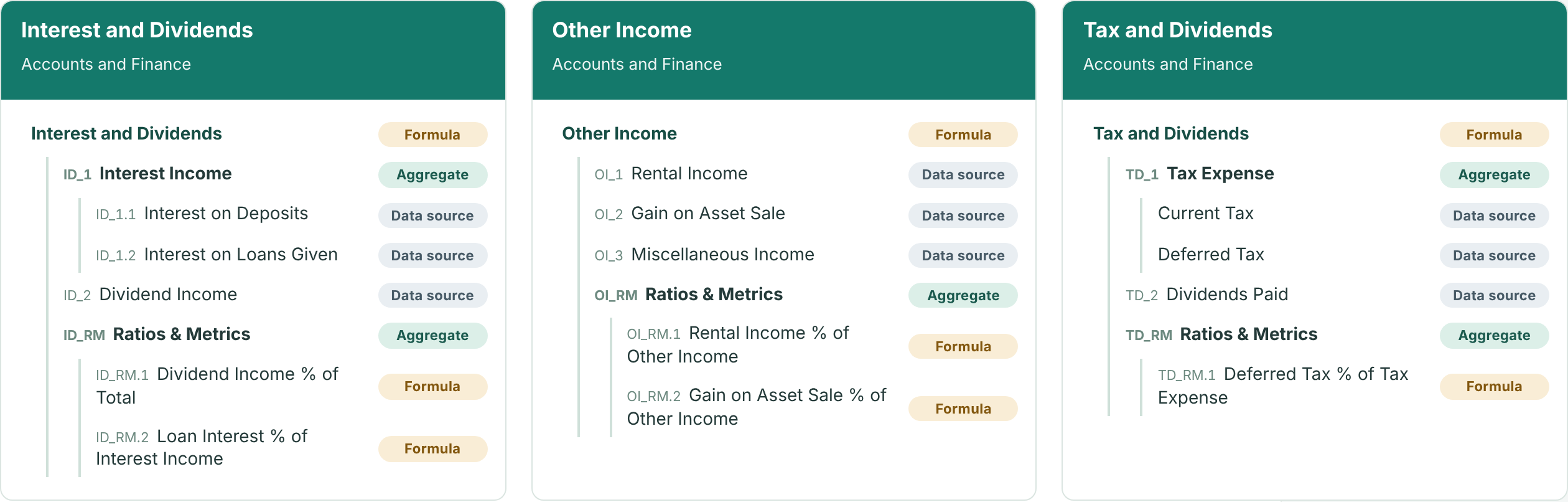
Aggregate groups the rows beneath it. Data source holds an input. Formula calculates a value or a ratio.
The rest of this post uses a sample model called Meridian & Atlas Group. Its five templates are attached to the members of a single anchor level, which here is Department, and each department only carries the templates that apply to it. Operating Expenses applies to every department, while Gross Margin applies only to the two sales departments, Retail Sales and Trade Sales. Midtown Branch looks like this:
| Department | Templates attached |
|---|---|
| Accounts and Finance | Operating Expenses, Interest and Dividends, Other Income, Tax and Dividends |
| General Administration | Operating Expenses |
| Marketing | Operating Expenses |
| Property | Operating Expenses |
| Retail Sales | Gross Margin, Operating Expenses |
| Trade Sales | Gross Margin, Operating Expenses |
A row only shows up where a member has it, and the group only combines the members that do, which is why Gross Margin comes entirely from the sales departments. Here’s how each template’s top row reaches the two organizations and the group in 2026:
| Template | Atlas Commerce Holdings | Meridian Retail Group | Group |
|---|---|---|---|
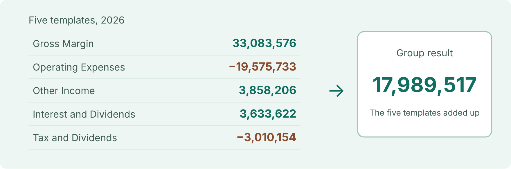
| Gross Margin | 14,047,762 | 19,035,814 | 33,083,576 |
| Operating Expenses | −8,695,060 | −10,880,673 | −19,575,733 |
| Other Income | 1,627,996 | 2,230,210 | 3,858,206 |
| Interest and Dividends | 1,556,987 | 2,076,635 | 3,633,622 |
| Tax and Dividends | −1,245,624 | −1,764,530 | −3,010,154 |
| All (group result) | 7,292,061 | 10,697,456 | 17,989,517 |
Everything reconciles. Gross Margin, for example, is 14,047,762 + 19,035,814 = 33,083,576, and the five templates together make up the group result of 17,989,517.
Every template row says how it should combine across the members it’s attached to. In Model Builder that’s the Rollup Aggregation column, which sits next to the Aggregation column that handles time. The idea behind it is Instance Aggregation, where an instance is simply one copy of a row for each member the template is attached to, such as each department.
The rule follows the metric, whatever kind of row it is, so a Data Source, a Data Input and a Formula row can each get whichever rule fits what they measure.
| Kind of row | Rollup rule | Why |
|---|---|---|
| Revenue, costs, units | Sum | Amounts simply add up across members |
| Prices and rates | Average | A price makes more sense as an average than as a total |
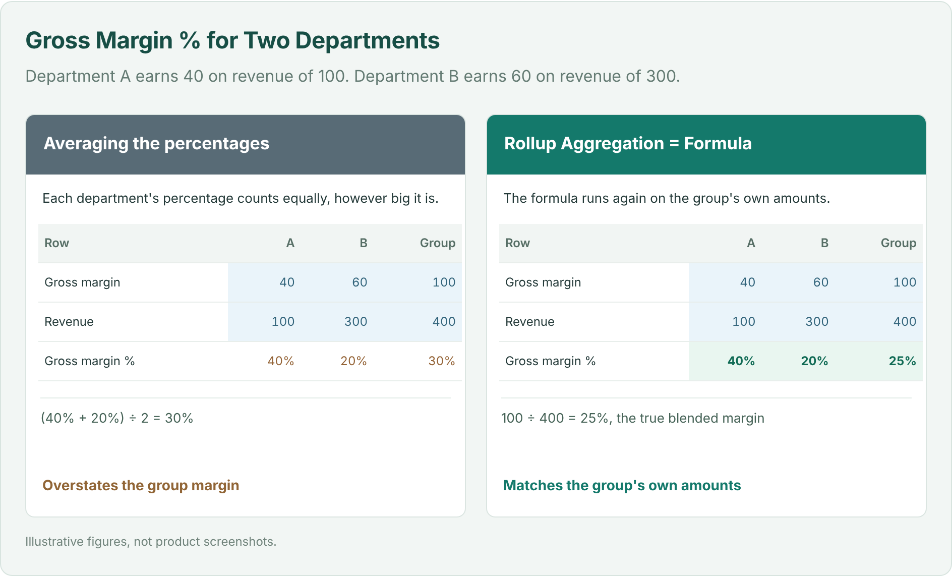
| Margin %, cost-to-income ratio | Formula | The ratio gets worked out again from the rolled-up amounts |
| Best or lowest value in a group | Maximum or Minimum | You want the benchmark across members |
You can’t add percentages together, and averaging them gives the wrong group figure. With Formula, the row’s own formula runs again at each level, using the amounts that level has rolled up, and that includes the group total.
Open Model → Row Model to get to Model Builder. Start by choosing the bottom-most layer you want your templates to apply to, which is Department in this sample model, and then build your templates and apply them conditionally.
Different people want to see different things. The CFO wants the group, a regional controller wants one organization and a branch manager wants their own branch, and none of them needs a separate model to get it.
A pivot is a view of the full model. Every level keeps calculating whatever is on screen, so pivoting away Organization, Region, Branch or Department only hides those rows and never stops their formulas, and the numbers regroup at whichever level you choose. Since a pivot is only a view, a new audience just means saving a new pivot.
Let’s start with the full model, with every level showing. The built-in All pivot has both Row Pivot and Column Pivot switched off.
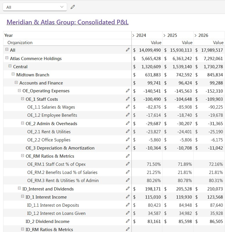
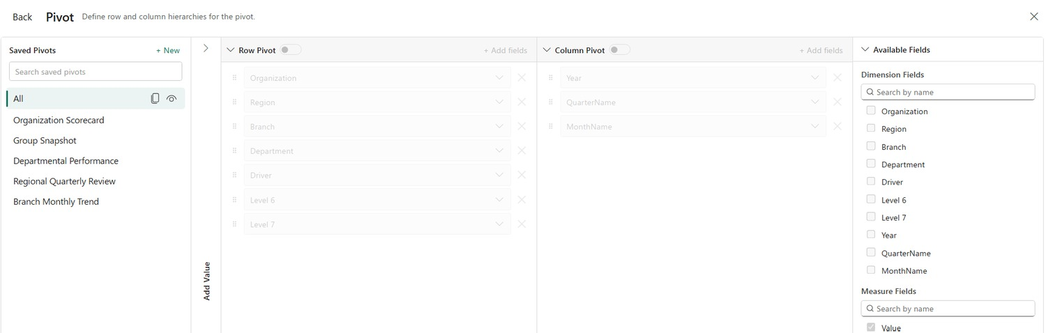
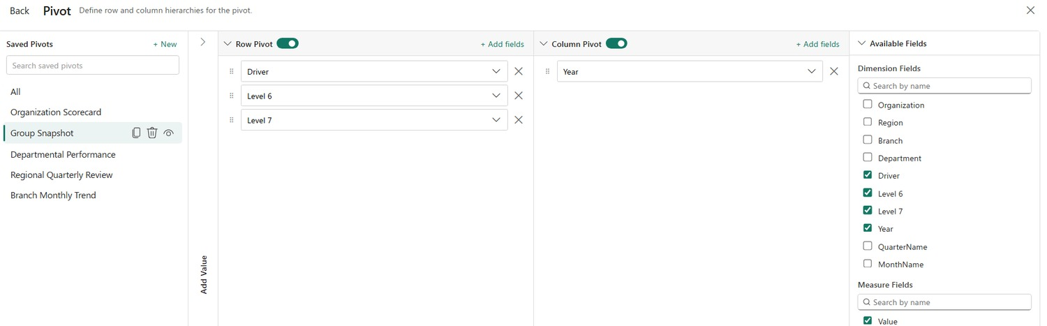
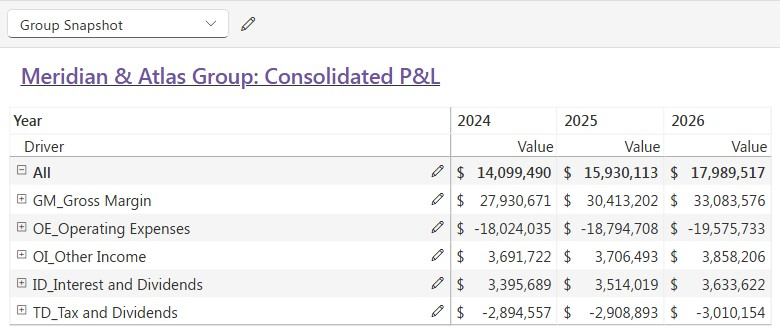
Saved pivots then give each audience its own arrangement of the same model. Group Snapshot keeps only the template rows, which appear under the Driver field, and leaves out Organization, Region, Branch and Department, so each template row combines every department that carries it.
Organization Scorecard keeps the Organization level and rolls up everything beneath it.
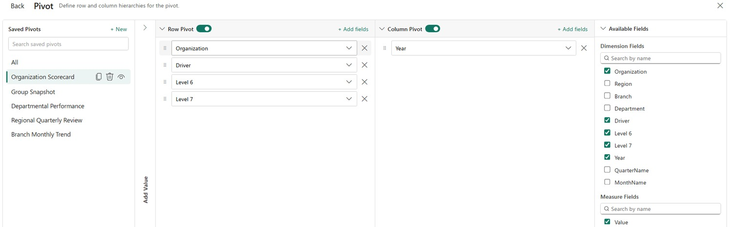
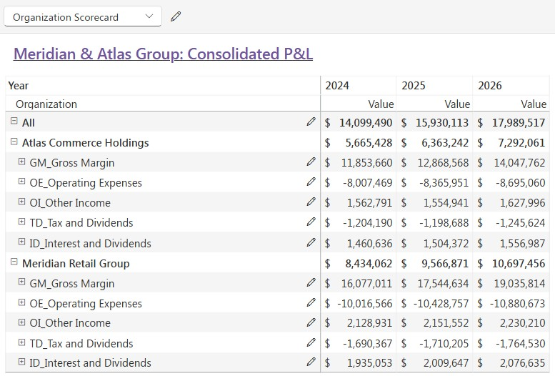
Whichever view you open, the group result is the same:
| View | Rows it shows | 2024 | 2025 | 2026 |
|---|---|---|---|---|
| Full model (All) | Every level, down to the template rows | 14,099,490 | 15,930,113 | 17,989,517 |
| Organization Scorecard | Organization, then the template rows | 14,099,490 | 15,930,113 | 17,989,517 |
| Group Snapshot | The template rows only | 14,099,490 | 15,930,113 | 17,989,517 |
You can also expand Year, Quarter and Month in the same view, so members and time roll up together.
Pivots work best as one saved view per audience, so that each person opens the same model at the level they manage. Setting up a view doesn’t need a rebuild or any manual consolidation, and people can switch between views with ease.
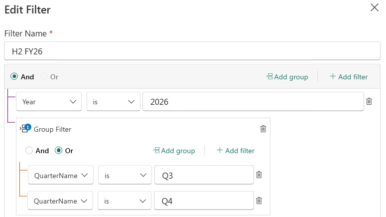
A pivot changes the level you look at, and a filter changes the scope. Say the CFO only wants the second half of 2026. The pivot stays exactly as it is, and every number simply follows the filter.
| Scope | Group result |
|---|---|
| 2026, full year | 17,989,517 |
| H2 FY26, Q3 (4,248,198) plus Q4 (6,238,672) | 10,486,870 |
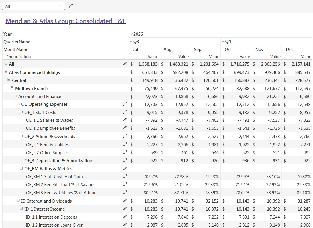
Because the filter works on the underlying model, every total and ratio is recalculated for that scope alone, and the pivot follows along. You also don’t need to bring a level back just to filter on it, so you can keep Region off the rows and still leave a few regions out.
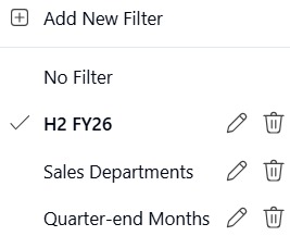
Filters work best as saved scopes for the cuts people keep asking for. A filter includes or excludes the data for you, so nobody has to remove rows by hand and then remember to add them back.
The real payoff comes from pairing a pivot with a filter. Organization Scorecard with H2 FY26 gives each organization lead a half-year view, and Group Snapshot with Sales Departments gives the board the sales result for the whole group.
Between them, the pivot, the filter and the rollup rules let you look at the group however you like, and the numbers still add up.
Setting it up takes three steps.
That’s really all there is to it. Pivots, filters and new members all work from that setup, and there’s nothing else to build or maintain.
You choose one anchor level, which here is Department, and a template attaches as a child of every member at that level, so Operating Expenses sits under every department. When a template should only apply to some members you add conditions, and that’s how Gross Margin ends up on Retail Sales and Trade Sales and nowhere else.
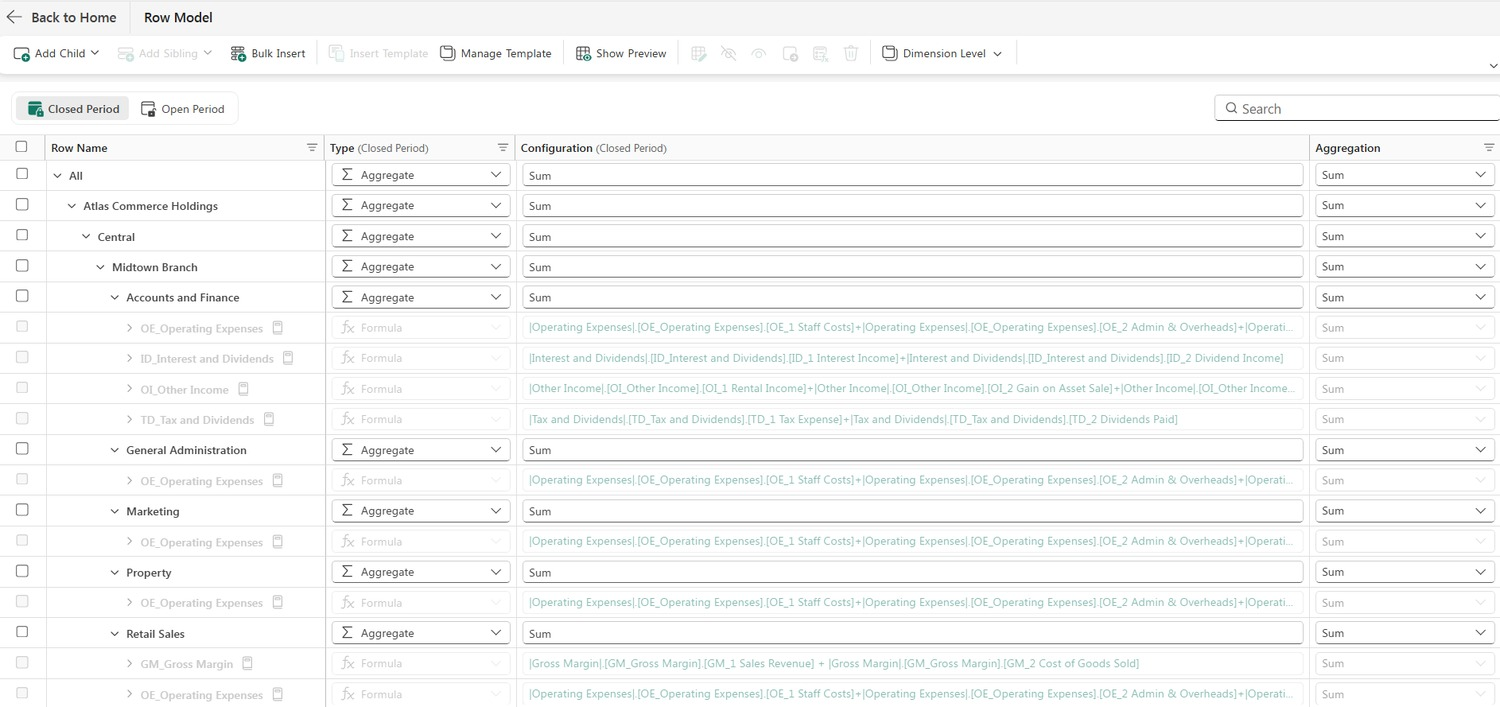
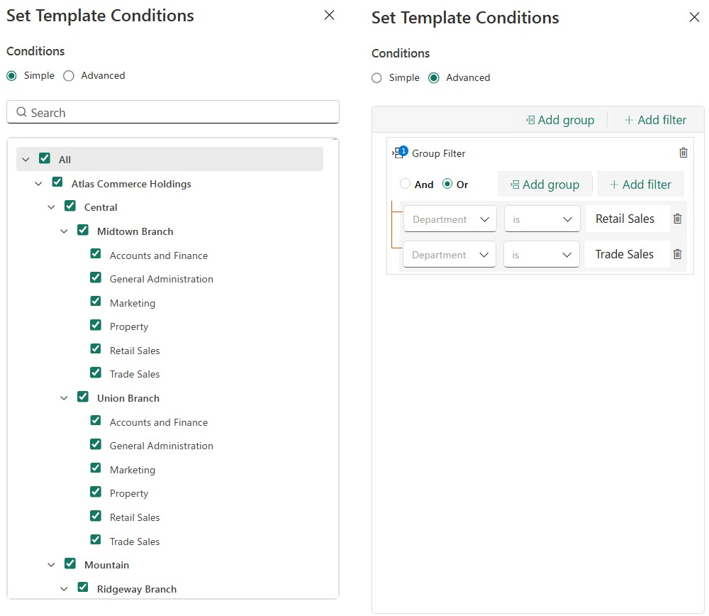
Since the rollup rules live on the template rows, nothing else has to change when the shape of the group does. A new dimension member, like a new region or division, sits under the anchor row and is consolidated automatically through its templates, and a row still only shows up where that member has it.
The setup also stays small however big the hierarchy gets. You list your metrics and say how each one rolls up, and there’s nothing to add together or structure by hand.
Consolidation Templates aren’t only for the close. The pattern fits any situation where many people need the same metrics at different levels of one hierarchy, and that includes group reporting across multiple legal entities. A few signs that it fits:
In each use case below, the levels sit on the pivot rows and each person reads the level they manage. Year, Quarter and Month can go on the column pivot as well, so every use case works period by period too.
| Use case | Pivot rows: level (read by) | Adds up (Sum) | Ratios, worked out at every level (Formula) |
|---|---|---|---|
| Group reporting and legal entities (after adjustments and eliminations) | Group (board and group CFO) › Region (regional finance leads) › Legal entity (entity controllers) › Department (department heads) | Revenue, costs, headcount | Gross margin %, cost-to-income ratio, cost per head |
| Sales performance | Company (sales head) › Region (regional leads) › Team (team leads) › Rep (individual reps) | Bookings, quota, pipeline | Quota attainment %, win rate, average deal size |
| Retail and franchise operations | Group (COO) › Region (area managers) › Store type (format leads) › Store (store managers) | Footfall, orders, revenue, floor area | Conversion rate, average order value, sales per square foot |
| Workforce and headcount | Company (HR head) › Division (division heads) › Department (department heads) › Team (team leads) | Headcount, leavers, payroll cost | Attrition %, cost per FTE, absence rate |
| Supply chain and logistics | Network (supply chain head) › Region (regional managers) › Hub (hub managers) › Route (route planners) | Shipments, units delivered, freight cost | On-time delivery %, fill rate, cost per shipment |
| Manufacturing and operations | Group (operations director) › Plant (plant managers) › Line (line leads) › Shift (shift supervisors) | Planned hours, downtime hours, units made, scrap units | OEE, scrap rate, yield % |
| Sustainability reporting | Group (sustainability lead) › Country (country heads) › Site (site managers) | Energy used, emissions, waste | Emissions per unit made, recycling rate |
| Projects and portfolio | Portfolio (PMO) › Program (program managers) › Project (project managers) | Budget, actual cost, effort | Percent complete, cost variance %, utilization |
| Real estate and facilities | Portfolio (asset head) › Region (regional managers) › Property (property managers) | Rentable area, occupied area, operating cost | Occupancy rate, cost per square foot, rent collected % |
Templates can differ by member type here too, just as Gross Margin does in the sample model. Flagship stores might carry footfall while online stores carry sessions, and call-center sites might carry handle time while field sites don’t. Customer support, marketing performance and healthcare operations follow the same pattern.
Group reporting across multiple legal entities is a natural fit as well. Each legal entity carries its own structure and the group view rolls them all up.
Most tools can show you a group total. What’s hard is rolling up rows that follow different rules, keeping the metrics right at every level, and doing it all over again whenever the hierarchy or the question changes. Here’s how the common approaches handle it, task by task.
| Approach | Task | Where it falls short | Consolidation Templates |
|---|---|---|---|
| Spreadsheets and pivot tables | Setup | You build and link a consolidation layer by hand | List your metrics and say how each one rolls up |
| Spreadsheets and pivot tables | Ratios at group level | Helper columns that get rebuilt at each level | The row’s own formula runs again at each level |
| Spreadsheets and pivot tables | New region or division | Rows and links added, then totals re-checked | It consolidates automatically |
| Spreadsheets and pivot tables | New view or scope | Another layout built, rows excluded by hand | Save a pivot or a filter |
| Spreadsheets and pivot tables | Who can maintain it | Mostly the people who built it | The rules sit on the row where everyone can see them |
| BI matrices and report visuals | Ratios at group level | Custom measures for each row and level | One rule, set on the row |
| BI matrices and report visuals | New view for an audience | A new report each time | Save a pivot |
| Multidimensional engines | Changing the layout | Results depend on calculation order, which the modeler has to manage | The pivot is just a view, so the logic doesn’t change |
| Planning platforms with per-line rollup settings | Different behavior by level or member | Helper lines or extra modules | Templates attach to members with conditions |
| Separate consolidation tools | Upkeep | A separate system to keep in step with planning | The rollup lives inside the planning model |
| Separate consolidation tools | Versions | More models and versions running in the background | One model behind every view |
The common thread is manual work that keeps coming back. With Consolidation Templates the logic is written once, on the row, and every view reads from it.
Intercompany adjustments and eliminations are a separate step. They’re done in other planning sheets for now, and PowerTable support is coming, with more on that further down. Once the final data is ready, Consolidation Templates show the reporting across every entity, level and scope.
At heart the benefit is the same for everyone: one model answers questions at every level, without rebuilds or manual consolidation. Here’s what that looks like for each audience.
| Audience | What they get | Why it holds |
|---|---|---|
| Board and CFO | One group view that ties to the detail, and an easy switch to any organization or scope | Pivots and filters are saved views on one model |
| Business and department managers | Their own level, ready to open, with ratios that are right | Each audience has a saved pivot |
| FP&A and analysts | More time on analysis, less on adding up or excluding rows by hand | The rollup rule is set once, and filters replace manual include and exclude |
| Model owners and IT | Very little to maintain as the business grows | New regions and divisions consolidate through their templates |
| Controllers and reporting leads | Totals that reconcile to the members beneath them | Each metric has one definition, and the templates do the consolidating |
Consolidation Templates are one part of a bigger plan for group and management reporting. Two roadmap items extend it further.
Disclaimer: This is a forward-looking roadmap. The items above are plans, and the exact release timing might vary.
Pick one set of metrics that your team rebuilds for each audience or every period, whether that’s the financial close, a sales scorecard or a store performance pack. Give each row a rollup rule that fits what it measures, then save a pivot for every view people ask for and a filter for every scope.
From then on, the group view, the regional view and the branch view all come from the same model, and each total reconciles to the members beneath it.
Feature details reflect Fabric Plan at the time of writing.
Available now with the Native Planning Engine. Driver-Based Planning in Fabric Plan relies on the Native Planning Engine’s file-based architecture in OneLake and is not supported by the previous planning engine. Turn on the engine at the tenant and workspace levels to start using it.
Your sales team revises its shipment forecast ahead of the holiday season. Operations expects higher delivery volumes, and finance needs to understand the cost impact.
The business relationship is straightforward: more shipments mean more delivery expense. Updating the plan should be just as straightforward.
In a spreadsheet, someone needs to connect the right cells, copy formulas across periods, check references, and maintain separate assumptions for different regions. In a planning application, a similar change may require additional model configuration before planners can use it. As the plan grows, these connections take more effort to maintain.
Driver-Based Planning lets you configure a relationship directly in your Fabric Plan sheet. Choose the row and measure you want to calculate, select the row and measure that will drive it, and define the operation. Keep the assumption visible in the grid, where planners can review and change it.
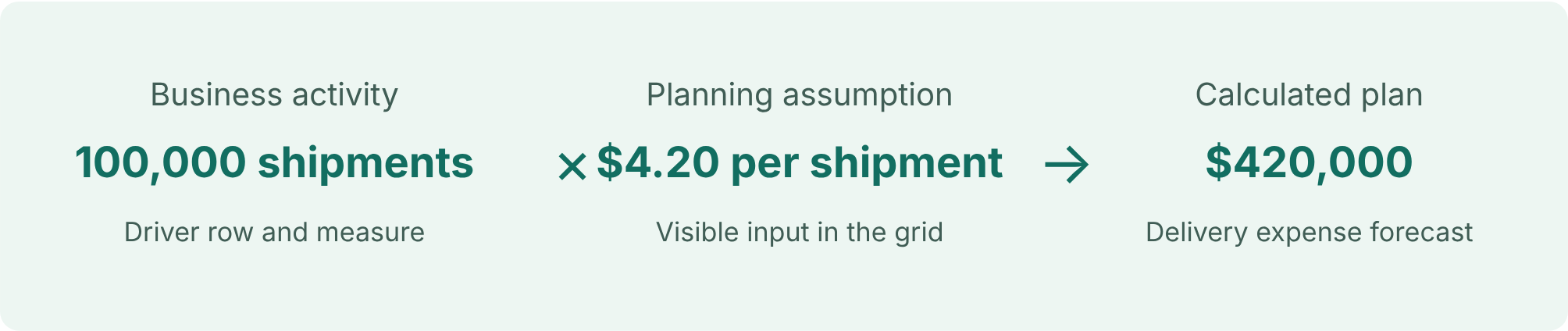
A logistics company is preparing its fourth-quarter operating plan. Delivery expense depends on forecast shipment volumes and an expected cost of $4.20 per shipment.
| Planning item | October | November | December |
|---|---|---|---|
| Forecast shipments | 100,000 | 120,000 | 180,000 |
| Cost per shipment | $4.20 | $4.20 | $4.20 |
| Delivery expense | $420,000 | $504,000 | $756,000 |
Entering the expense estimates separately creates unnecessary work whenever volumes change. Connecting them to the shipment forecast keeps the business assumption consistent.
If November’s volume increases from 120,000 to 140,000 shipments, delivery expense becomes $588,000 at the same rate. Finance can focus on the impact of that change instead of rebuilding the calculation.
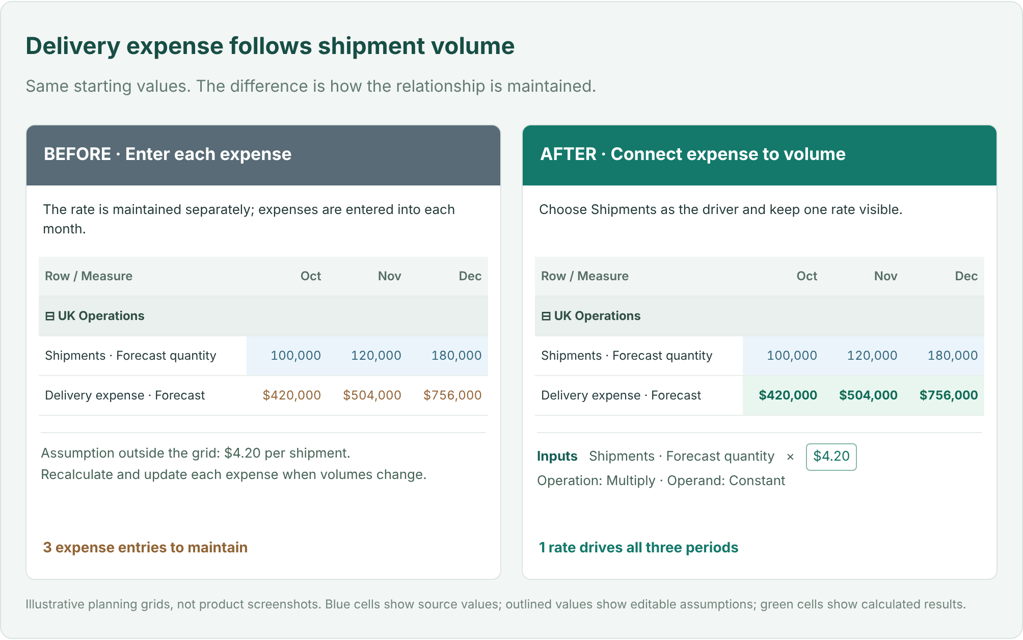
A row can contain several measures, such as quantity, price, revenue, and forecast. Selecting a row alone does not identify which value should be calculated. Driver-Based Planning makes the destination and source explicit.
| Configuration | Logistics example |
|---|---|
| Destination row | UK Operations → Delivery expense |
| Destination measure | Forecast |
| Driver row | UK Operations → Shipments |
| Driver measure | Forecast quantity |
The measures can differ: a quantity measure can drive an expense measure. The destination must be an eligible Data Input target; the driver can use an available source measure, including a native measure.
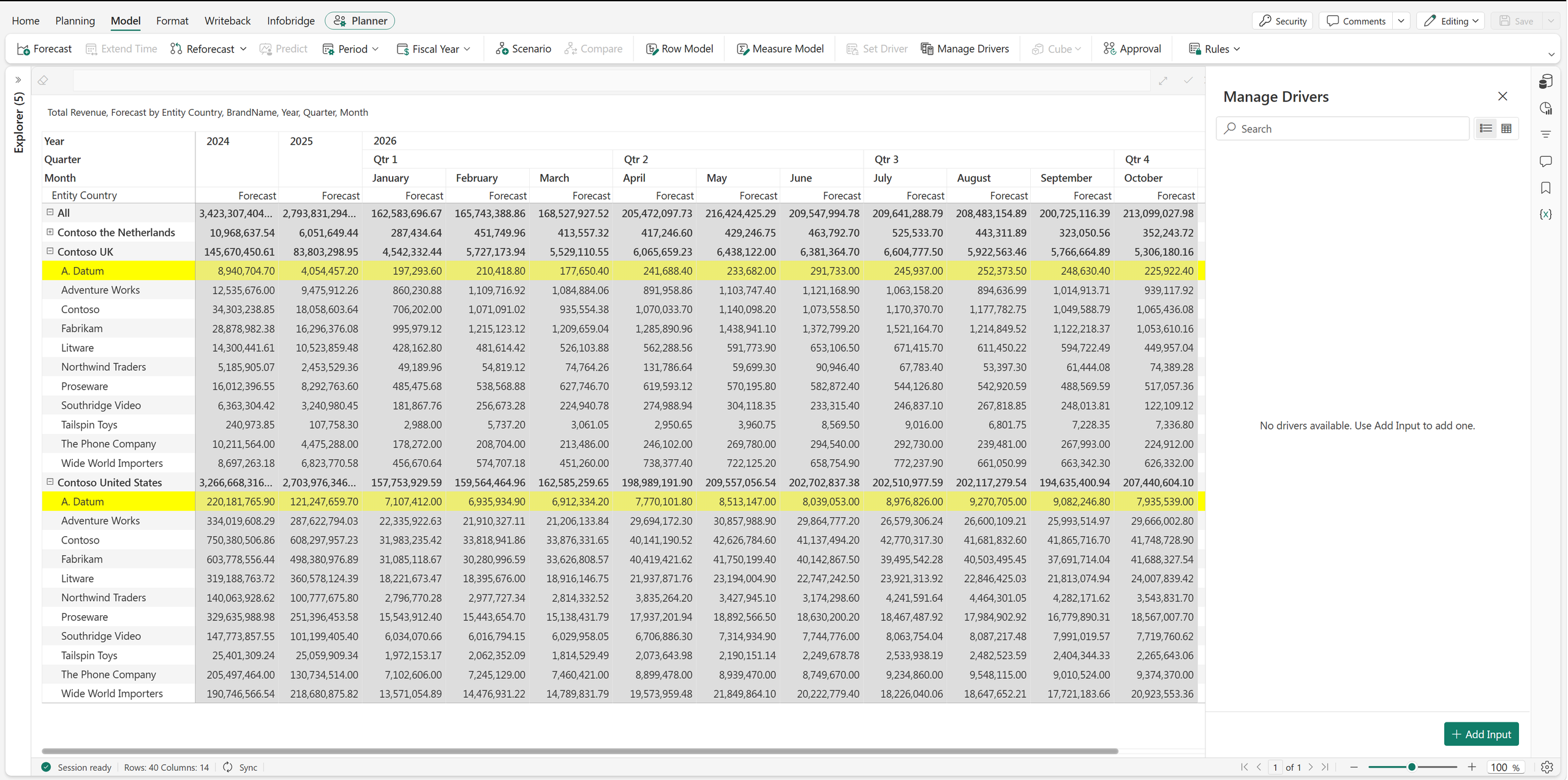
Open Model → Manage Drivers → Add Input and select the destination row from the hierarchy.
All of these settings are in the Set Driver panel.
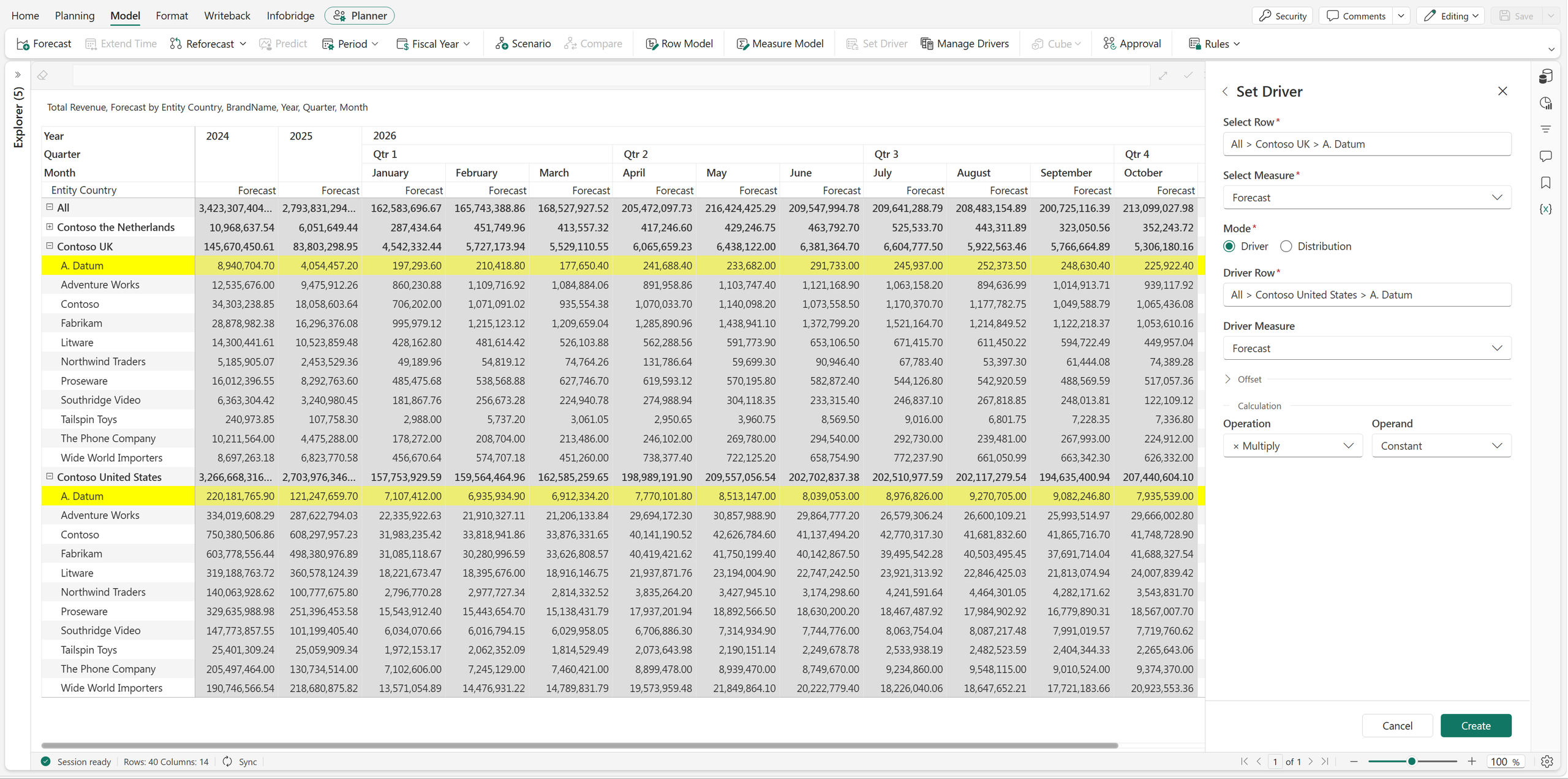
With Constant, one visible assumption applies across the periods governed by the rule. Planners can see and adjust the rate without searching through cell formulas.
Delivery rates often rise during peak season. The logistics company expects a November surcharge and a higher December rate. A single constant no longer represents the business.
Change Operand to Value by Month. Fabric Plan displays input boxes across the periods. Enter the appropriate delivery rate for each month.
| Planning item | October | November | December |
|---|---|---|---|
| Forecast shipments | 100,000 | 120,000 | 180,000 |
| Monthly delivery rate | $4.20 | $4.60 | $4.80 |
| Delivery expense | $420,000 | $552,000 | $864,000 |
The quarter’s expense is now $1,836,000, compared with $1,680,000 at a constant $4.20 rate. The additional $156,000 has a clear explanation: the volumes are unchanged, but the November and December rates are higher.
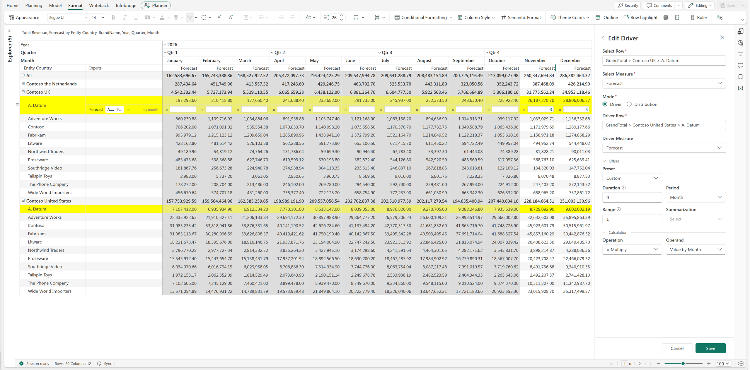
This is useful for seasonal costs, scheduled price changes, and productivity assumptions. The relationship stays consistent while the inputs reflect the business calendar.
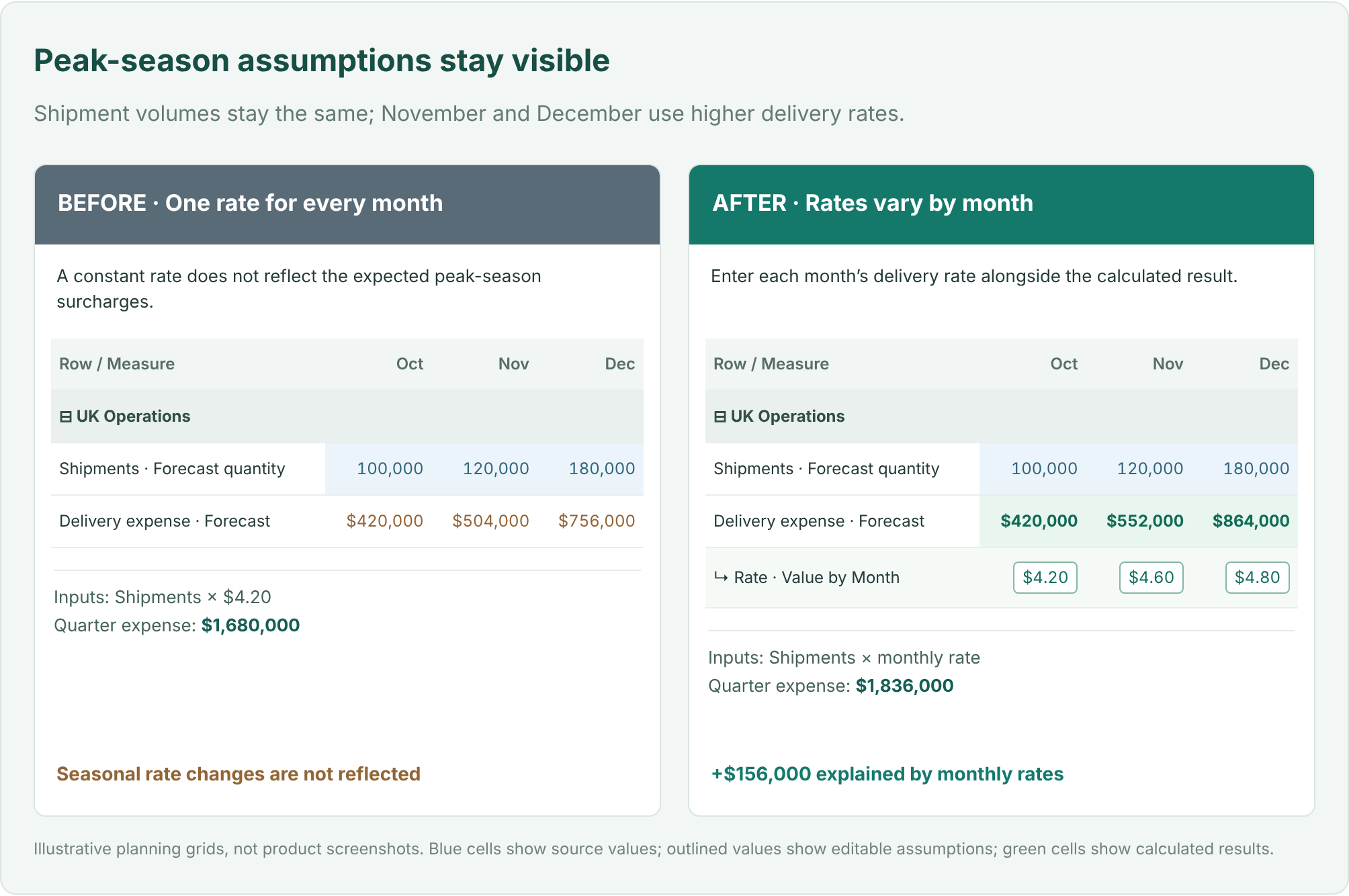
Driver mode supports five operations. Each rule applies one operation to the selected driver value, using a constant or a period-specific operand.
| Operation | Business example | Result |
|---|---|---|
| Multiply | Shipments × cost per shipment | 100,000 × $4.20 = $420,000 |
| Percentage | Revenue at a commission rate | $2,000,000 at 3% = $60,000 |
| Divide | Labor hours ÷ hours per FTE | 16,000 ÷ 160 = 100 FTE |
| Add | Baseline demand + extra units | 100,000 + 5,000 = 105,000 |
| Subtract | Gross demand − canceled units | 100,000 − 2,000 = 98,000 |
Taking a percentage and increasing a value by a percentage are different questions. A 3% commission is 3% of revenue. A 3% uplift can be expressed by multiplying the baseline by 1.03.
Not every plan should follow the current period’s value. You may want to carry forward an earlier month, smooth recent volatility with an average, or use a total across a historical window.
Open Offset to choose a preset.
| Preset | What it does | Input |
|---|---|---|
| Prior Period | References an earlier period | Go back |
| Rolling Average | Averages values across a window | Window |
| Rolling Total | Totals values across a window | Window |
| Custom | Sets the reference window explicitly | Duration, Period, Range, Summarization |
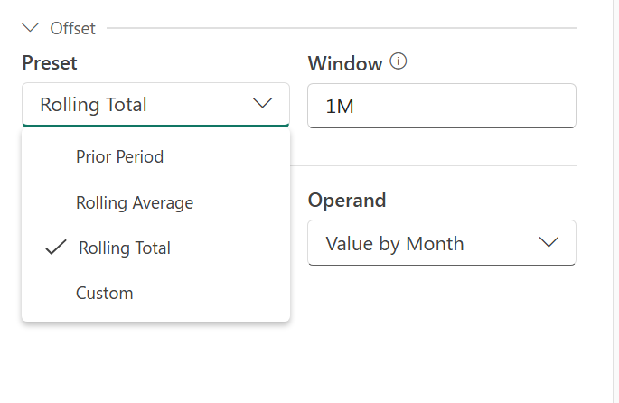
For Prior Period, enter 1M to go back one month, 1Q for one quarter, or 1Y for one year. Rolling Average and Rolling Total use a Window input to specify the period span.
Suppose finance wants November’s baseline delivery expense to reflect the average shipment volume from July through October.
| Historical month | Shipments |
|---|---|
| July | 80,000 |
| August | 90,000 |
| September | 110,000 |
| October | 100,000 |
| Four-month average | 95,000 |
Select Custom and configure Duration = 1, Period = Month, Range = 4, and Summarization = Average. Keep the operation as Multiply and enter a constant of 4.20.
For November, Duration moves the reference point back to October. Range includes four consecutive months ending there: July, August, September, and October. The average is 95,000 shipments, so the baseline expense is $399,000.
Duration determines how far back to look. Range determines how many periods to include. Summarization combines those values using Average, Sum, Lowest, or Highest. The selected historical value then feeds the calculation.
The logistics company has approved a $900,000 quarterly warehouse support budget. Finance wants to phase that amount according to expected shipment activity rather than divide it equally.
| Planning item | October | November | December | Total |
|---|---|---|---|---|
| Forecast shipments | 100,000 | 120,000 | 180,000 | 400,000 |
| Share of quarter | 25% | 30% | 45% | 100% |
| Support budget | $225,000 | $270,000 | $405,000 | $900,000 |
Choose the destination row and measure, then switch Mode to Distribution. Choose By Row and select the reference that supplies the shipment weights. Enter the amount to distribute across the relevant periods.
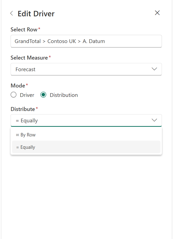
With Equally, the budget would be $300,000 in each month. With By Row, December receives $405,000 because it represents 45% of the quarter’s shipments. The total remains $900,000; the timing reflects the activity it supports.
Offsets also work with the reference values used for distribution weights. You can use an earlier activity pattern when that is a better basis for phasing the budget.
Driver mode calculates a value from a business relationship. Distribution mode spreads an amount across periods.
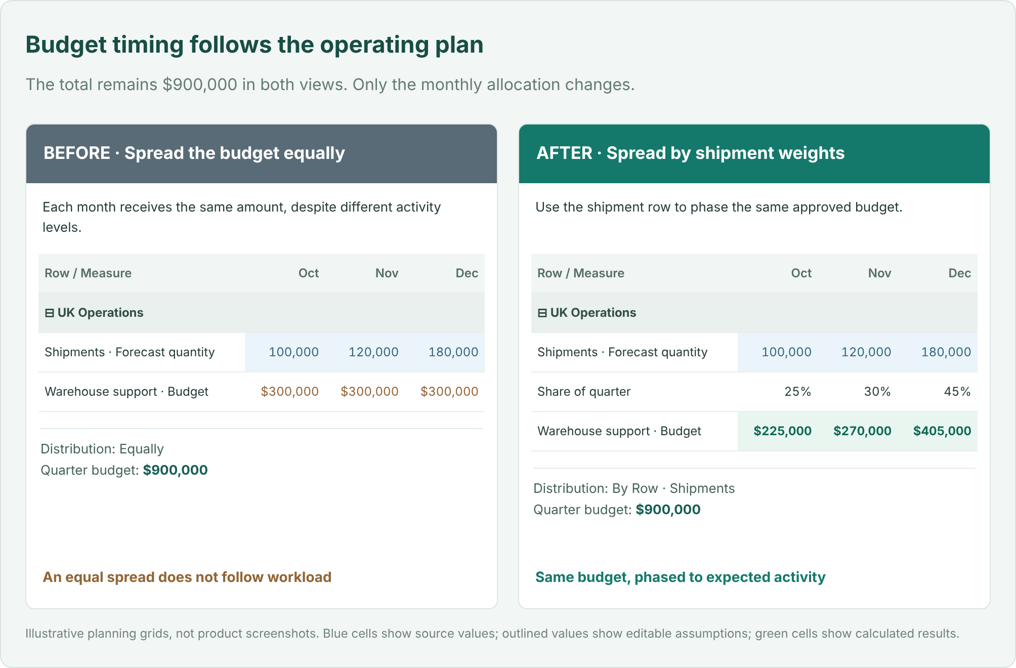
When the source, operation, and assumption are visible together, it becomes easier to explain a change. Operations can challenge the cost per shipment. Finance can identify which months include a surcharge. Regional managers can see how the budget follows expected activity.
Driver-Based Planning works with both Row Model and Measure Model sheets. Where a row has multiple eligible Data Input measures, each can have its own independent driver configuration.
For a driver-governed result, update the driving value or its assumption. Directly typing over that result does not reverse-solve the driver. This keeps the relationship explicit.
Start with one relationship your team already understands: delivery expense driven by shipments, commissions driven by revenue, or labor requirements driven by workload. Select the destination, choose its driver, and enter the assumption. Then change the source or rate and review the resulting plan.
Spend less time maintaining the connections between numbers, and more time deciding whether the assumptions behind them are right.
Feature details reflect Fabric Plan at the time of writing.
Available now for all Plan items. Anchoring Measures does not require the Native Planning Engine; it works with both the Native Planning Engine and the previous planning engine.
A product’s unit price belongs beside the product. A regional assumption belongs where the regional team maintains it. An executive profitability metric belongs in the summary where leaders review it.
But add those measures to a hierarchical grid, and they can appear everywhere: at region totals, category subtotals, individual SKUs, and every expanded period. The grid treats them alike even though they serve different business purposes.
Anchoring Measures in Fabric Plan lets you choose the row and column levels where each measure belongs. It works with Power BI Measures, input measures created in the plan, and formula measures created in the plan. For input measures, the anchor also defines where users can enter values directly.
You can build one view that shows product details, business assumptions, and executive results at their appropriate levels, with fewer repeated measures to navigate.
Imagine a retailer planning across Region → Category → SKU, with Year → Quarter → Month on columns. The plan includes quantity, unit price, standard unit cost, price uplift, revenue, and EBITDA margin.
Those measures answer different questions. A planner needs quantity at SKU and month. A pricing team maintains an annual uplift by region. Leadership reviews quarterly EBITDA margin by region. A price displayed at the regional subtotal may be technically calculated by the model, but it is not the product price the planner needs.
Without control over placement, teams often accept a cluttered grid, build separate summary and detail reports, or maintain assumptions in a separate spreadsheet block connected to the plan by formulas. Users must remember which repeated values are meaningful and which cells they should update.
Anchoring makes that intent part of the grid configuration. Here are three realistic ways it helps.
A retailer sells two products with centrally maintained prices and standard costs:
| Product SKU | List price per unit | Standard cost per unit |
|---|---|---|
| Travel Mug TM100 | $24 | $9 |
| Water Bottle WB200 | $32 | $12 |
In this example, each SKU’s list price and standard cost are the same across regions. These are Power BI Measures from the Power BI semantic model.
When the measures repeat throughout the hierarchy, the grid also presents them at Category and Region subtotals. Whether the underlying measure returns an average, another aggregate, or a blank, that placement distracts from the intended question: What is the price or cost of this SKU? A regional subtotal is not another product with its own list price.
Teams may work around this with a separate product reference report or special display logic in their measures. That adds maintenance just to control where a number appears.
Anchor List Price and Standard Unit Cost to the SKU level. Users see those measures at product detail, while Region and Category subtotals focus on totals such as quantity, revenue, and gross profit. Hide the non-anchored instances to remove those price and cost measures from the subtotal levels.
The SKU’s $24 price still comes from the Power BI measure. Anchoring controls its placement; it does not force prices to be identical across regions or alter the DAX calculation. The shared regional price is already a rule of this example’s semantic model.
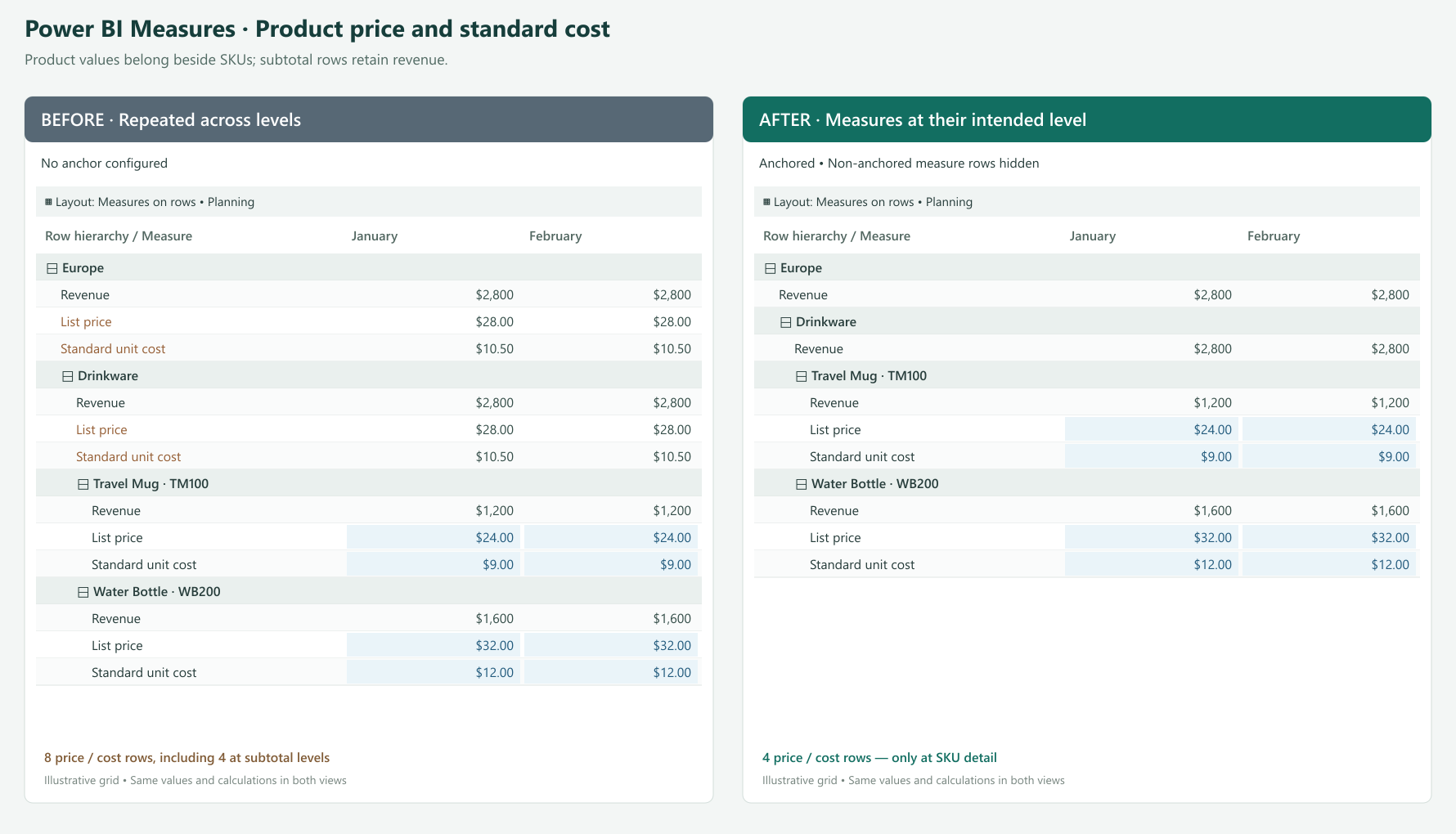
Open Manage Rows (Show Rows on the ribbon) or Manage Columns, locate the Power BI Measure, and click its anchor icon. In Anchor Measure, select the SKU dimension under Row Dimension, then apply the settings. Configure non-anchored instances to be hidden for the product-detail presentation.
The same approach is useful for measures such as standard weight per unit or price per pack when their meaningful reporting level is an individual product.
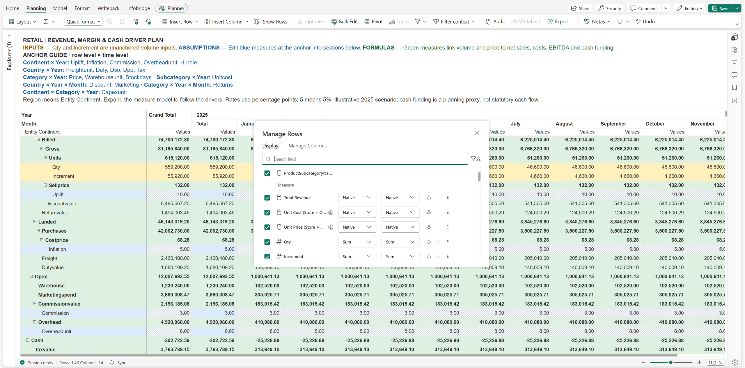
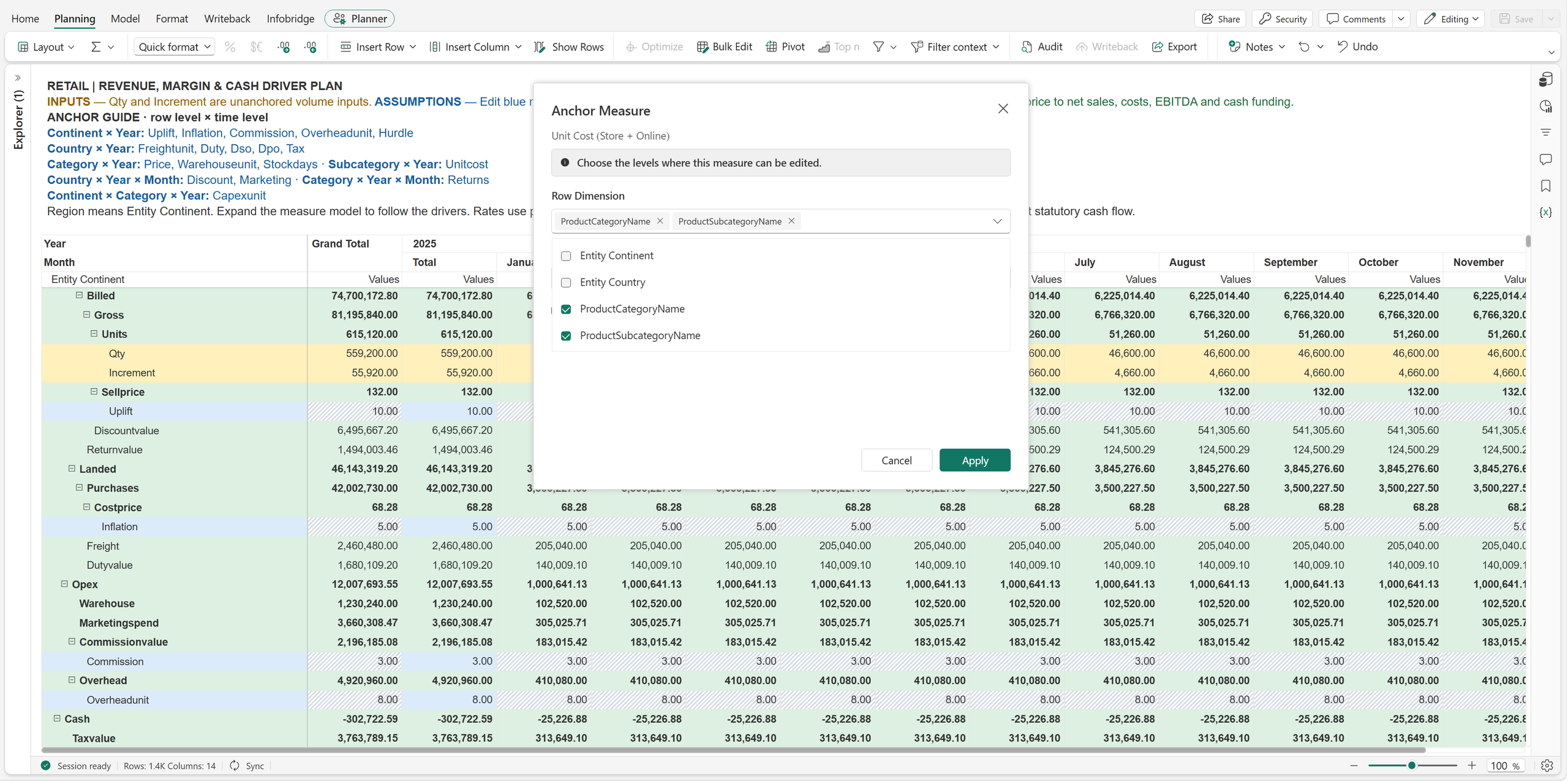
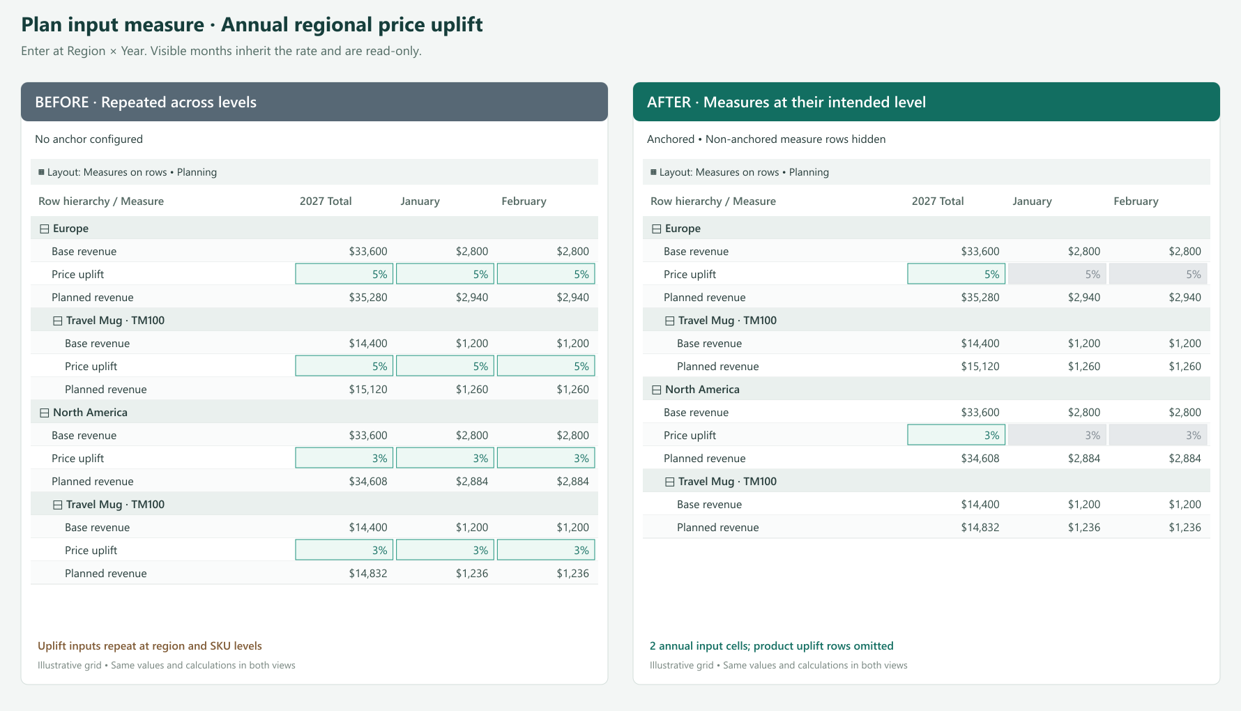
A pricing team agrees on an annual price uplift of 5% for Europe and 3% for North America. The sales plan contains hundreds of SKUs and twelve months of detail.
If the uplift is available for direct entry throughout the detail, users have many places to maintain a decision made once per region and year. They may copy the rate across cells or maintain a separate assumptions block above the plan. It becomes harder to tell whether a different value is intentional or an accidental override.
Anchor the Price Uplift input measure to Region × Year. Europe has one annual input point for its 5% assumption; North America has another for 3%. Users enter the values at the corresponding year subtotal.
With the existing distribution configured to repeat the rate, eligible detail receives the regional assumption. A product with a base price of $24 therefore has a planned price of $25.20 in Europe and $24.72 in North America, using:
Planned price = Base price × (1 + Price uplift)
The formula and distribution produce those values. The anchor makes the location for maintaining the assumption explicit. Monthly instances that remain visible are read-only; they are not separate places to override the annual policy.
An annual assumption belongs in the annual subtotal, not January. A quarterly assumption belongs in the quarter subtotal.
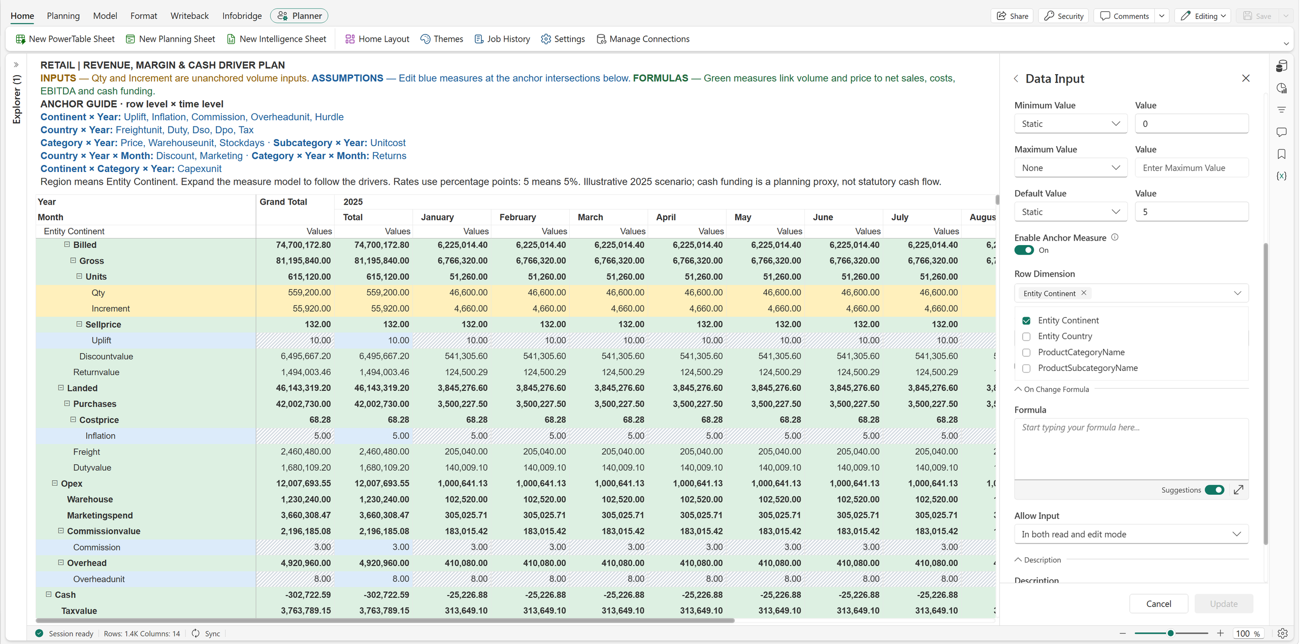
| Planning decision | Anchor | What users maintain |
|---|---|---|
| Annual salary increase | Year only | One annual policy shared across the employee plan |
| Regional benefit rate | Region × Year | One annual rate per region, such as 22% or 26% |
| Seasonal demand uplift | Year × Quarter only | One quarterly assumption shared across products and regions |
| Monthly promotion | Country × Year × Month | A discount assumption that varies by country and month |
| Inventory policy | Product category × Year | Annual target stock days for each category |
Neither row nor column selection is individually mandatory. With anchoring enabled, select at least one dimension overall. A time-only seasonal factor can leave Row Dimension empty. A factor that varies only by region can leave Column Dimension empty.
A regional management view includes Revenue, EBITDA, and EBITDA Margin. Users can expand the same grid to inspect categories and SKUs, but leadership wants profitability measures at the regional quarterly summary.
Showing EBITDA and EBITDA Margin beneath every SKU makes operational detail harder to scan. It can also encourage readers to interpret product-level profitability when some operating expenses are managed at a broader level. Teams may maintain a separate executive report simply to keep those measures out of the detail view.
Anchor the plan’s formula measures EBITDA and EBITDA Margin to Region × Year × Quarter. If Region is the top row level, those measures appear at the top business summary level for each region. SKU detail can focus on quantity, price, and revenue.
For example, Europe has quarterly revenue of $2.4 million and EBITDA of $360,000. Its existing formula calculates:
EBITDA Margin = EBITDA ÷ Revenue = 15%
Anchoring places that 15% where leadership reviews the result. It does not average displayed SKU percentages or change how the formula evaluates. Hiding detail instances also does not remove the data or dependencies needed to calculate the summary.
Use the same pattern for Profit Margin or Operating Profit at a selected management level. Choose the highest business dimension you want to present, such as Company, Business Unit, or Region, together with the relevant period.
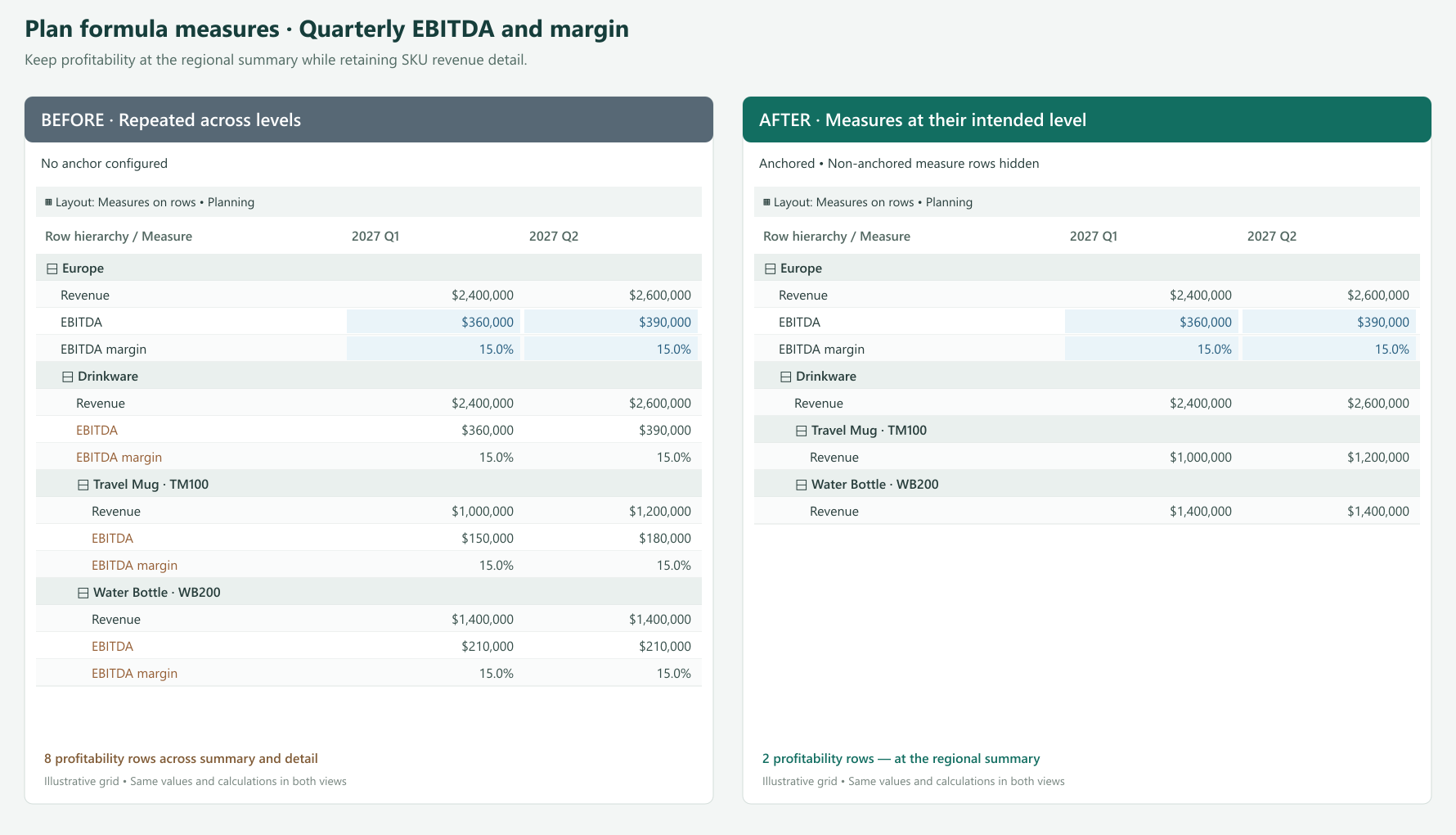
Open the formula measure’s anchor settings through its configuration or the anchor action in Manage Rows / Manage Columns. Select Region as the row dimension and Year and Quarter as the column dimensions. Apply the settings and hide non-anchored instances for the summary-focused presentation.
The formula remains calculated and read-only. Anchoring does not make a formula measure or a Power BI Measure directly editable, even when the shared dialog describes where a measure can be edited.
Show non-anchored instances when users need to follow an assumption into the detail; for input measures, these cells remain read-only. Hide them when the repeated measure adds no useful information.
A regional assumption need not have its own input row under every product in a measures-on-rows layout. A quarterly assumption need not add an input measure column beneath every month in a column layout. Hiding removes unnecessary instances where the layout permits while calculations continue to use the underlying values.
Read-only detail can still receive updates through the existing allocation or distribution process from a valid editable anchor. Normal permissions and locking rules continue to apply. Anchoring controls placement and entry locations; aggregation and allocation settings determine how values are distributed and rolled up.
| Measure type | Example | Appropriate placement | User interaction |
|---|---|---|---|
| Power BI Measure | List price or standard unit cost | SKU detail | Read the existing model value |
| Input measure in the plan | Annual regional uplift | Region × Year subtotal | Enter the assumption at the anchor |
| Input measure in the plan | Quarterly seasonality | All rows × Year × Quarter | Maintain one shared period assumption |
| Formula measure in the plan | EBITDA or profit margin | Management summary × reporting period | Review the calculated result |
Start with a measure that appears in too many places. Put it at the level where it is useful, expand the grid, and check how the detail reads. Then apply the same approach to other measures in the plan.
Product facts at product detail. Assumptions where decisions are made. Results where the business reviews them. Anchoring Measures brings those needs together in one planning and reporting view.
Feature details reflect Fabric Plan at the time of writing.
A plan rarely stops when the numbers are submitted. With writeback event triggers, a writeback can refresh reports, feed downstream systems and alert the right people, configured from the planning UI with no code. The loop from plan to action closes entirely within Fabric.
In this article:
Before Event Triggers, the steps after a writeback were manual or needed external plumbing: someone refreshed the report, re-ran a pipeline or called an API from an Azure Function. Now the plan starts that work itself, the moment the data lands, using the Fabric items your data team already runs.
The result: reports show approved numbers within minutes, downstream systems get the plan without a hand-off, and failures reach someone who can fix them.
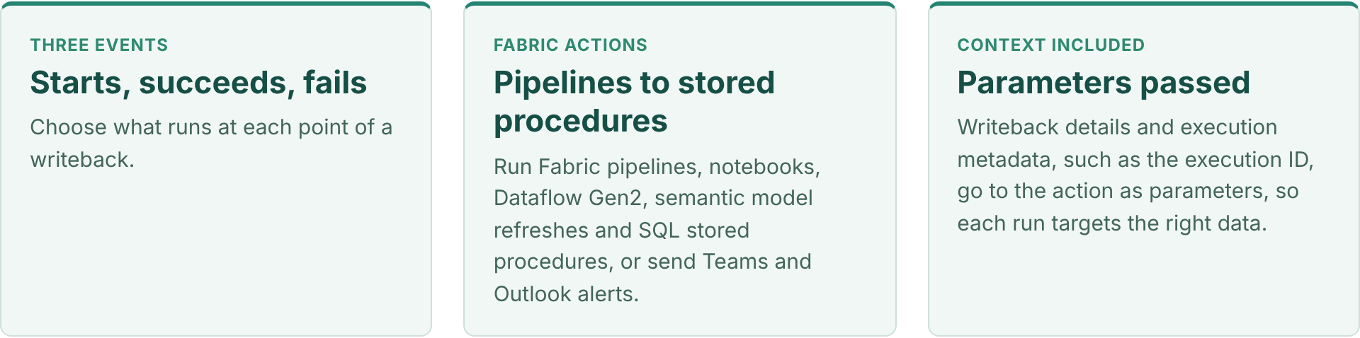
| When a writeback… | Typical actions | Example |
|---|---|---|
| Starts | Stored procedure, Teams or Outlook notification | Snapshot the current destination table before it changes, or tell data owners a load is under way |
| Succeeds | Semantic model refresh, pipeline, notebook, Dataflow Gen2, stored procedure, notification | Refresh the variance report, push the approved budget to the ERP, or recalculate a downstream allocation |
| Fails | Teams or Outlook notification, stored procedure | Alert the plan administrator with the error details and log the failed run |
You can configure several triggers on one planning sheet, so different automation paths run for different events, and run actions in sequence, such as a stored procedure followed by a semantic model refresh.
Demo, about 3 minutes: set up a trigger that runs a pipeline after a successful writeback, pass the execution ID as a parameter, chain a stored procedure with a semantic model refresh, and check each run in the trigger logs. Also on the Fabric Plan community.
Each one replaces a manual step that usually follows a planning cycle.
On succeeds, refresh the semantic model that holds plan versus actuals, so the variance report shows the new plan without waiting for the next scheduled refresh. See it end to end in Planning Decision to Business Action.
Once the plan clears approvals and is written back, run a Fabric pipeline on succeeds that copies the approved version to the ERP or a finance data mart, passing the scenario and version as parameters.
On succeeds, run a stored procedure or notebook that rebuilds allocations, aggregates or derived tables that depend on the plan, then refresh the semantic model that reports on them.
On fails, send a Teams or Outlook message to the plan administrator with the writeback details, so issues are fixed before the deadline.
Event Triggers are configured on the planning sheet, after a writeback destination exists.
Set up writeback to Fabric SQL or OneLake for the planning sheet. See writeback to OneLake and the Planning 103 – Writeback video.
From the planning UI, add a trigger and choose the event: when the writeback starts, succeeds or fails.
Pick the Fabric item to run and its connection, such as a pipeline, notebook, Dataflow Gen2, semantic model refresh or stored procedure, or a Teams or Outlook notification.
Pass writeback details and execution metadata, such as the execution ID, to the action, so it processes only what changed.
Run a writeback on a test version and confirm each action ran in the trigger logs, then add more triggers for other paths.
PowerTable too. PowerTable Automations can run stored procedures from a Fabric SQL database, passing values from the record that triggered them, alongside no-code create, update and find-record actions. Watch Execute Stored Procedure Action in PowerTable Automations and Setting Up Automations in PowerTable.
Pick the one task that always follows a writeback today, usually a report refresh, and make it an Event Trigger. Add the failure alert at the same time.
Sources
Feature details reflect published Fabric Plan updates at the time of writing.
The Native Planning Engine stores planning data and application metadata as files in OneLake. That one architectural shift, together with optimizations across the product, makes Fabric Plan faster from the first click to the final writeback.
This is Part 3 of our three-part Native Planning Engine series, covering the Fabric Plan performance improvements beyond calculation and writeback. Part 1 introduces the Native Planning Engine, and Part 2 covers writeback to OneLake.
Covered in Parts 1 and 2: 10× more scale (12M cells), 10× faster calculation and up to 13× faster writeback.
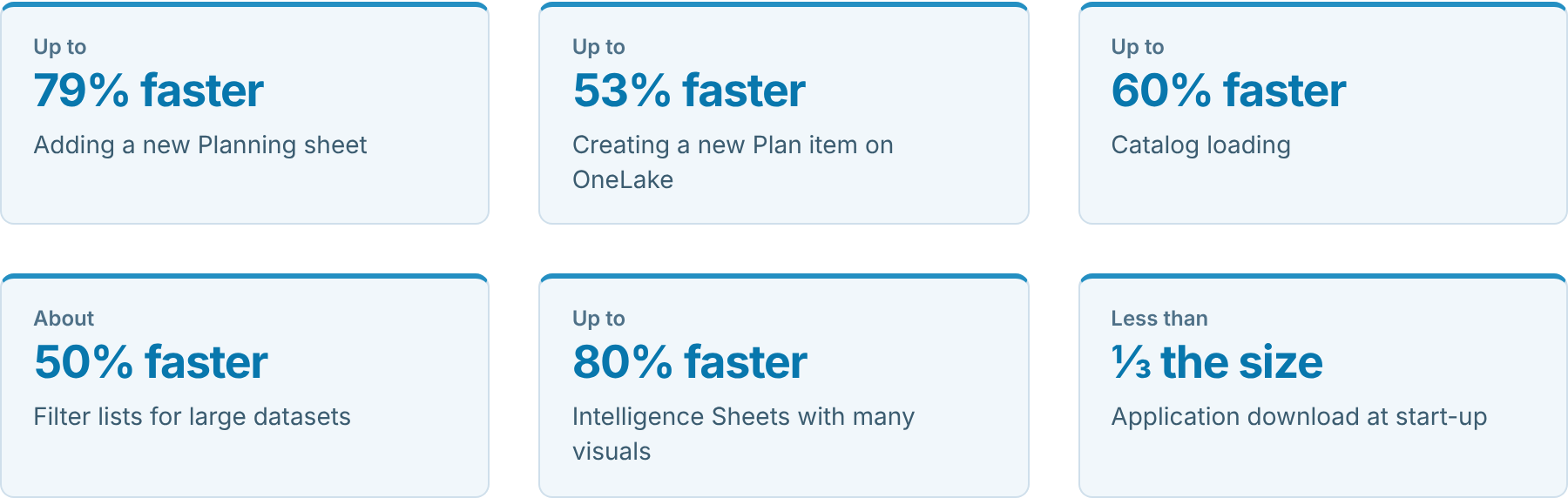
Figures come from our testing. Performance varies with workload, model design, data size and capacity.
With the Native Planning Engine, planning data and application metadata are stored as files in OneLake, and Plan items no longer need a separate system database. The benefits go well beyond the calculation and scale gains in Part 1 and the writeback gains in Part 2: creating and opening Plan items, adding Planning sheets and returning to views you use often are all faster too.
We also optimized start-up, the catalog, filters and Intelligence Sheets. Some of these improvements reach every Plan item; the full set comes with the Native Planning Engine and OneLake.
In this article:
The same everyday tasks, from launch to writeback, before and after the Native Planning Engine and OneLake.
| What you do | Before | After | Change |
|---|---|---|---|
| Launch Fabric Plan | A large application to download first | A compact package that loads quickly, even on slower networks | Less than ⅓ the size |
| Create a Plan item | Set-up took about twice as long | Ready for planning in about half the time | Up to 53% faster |
| Open a Plan item | Slower to open | Opens up to a third sooner | Up to 33% faster |
| Add a Planning sheet | Adding a sheet took up to five times as long | New sheets are ready in a fraction of the time | Up to 79% faster |
| Browse the catalog | The full catalog loaded up front | Each section loads as you open it | Up to 60% faster |
| Open a filter | Long member lists took time to appear | Lists appear with only the members you need | About 50% faster |
| Plan at scale | Up to 1.2 million cells in aggregate | Up to 12 million cells in aggregate (Part 1) | 10× more scale |
| Calculate the plan | Calculations on the previous planning engine | In-memory calculation on the Native Planning Engine (Part 1) | 10× faster |
| Load an Intelligence Sheet | Visuals competed for shared resources while loading | Visuals load side by side without waiting on each other | Up to 80% faster |
| Return to a view you use often | Data was fetched again each time | A fast local copy is used first | Faster repeat visits |
| Write back results | SQL-based writes | File-based Delta Parquet writes directly to OneLake (Part 2) | Up to 13× faster |
What it means for your team: less waiting during planning sessions, more scenarios tested before a deadline, and a tool that more people keep using.
Some of the result depends on how your environment is set up. These four steps make the biggest difference.
The file-based architecture is what unlocks the full set of improvements in this blog. Plan items still on the previous planning engine miss many of them.
Turn on Store new Plan items in OneLake at the tenant and workspace levels, start with new Plan items, then migrate your existing ones gradually. Part 1 walks through each step.
Saving planning results to OneLake makes everything above even more effective. Your plans, forecasts and assumptions sit in one governed place, and reporting across Fabric reads them directly.
File-based Delta Parquet writes to OneLake are about 5–6× faster than SQL-based writes at typical volumes and up to 13× faster at 12M cells. Fabric SQL remains a fully supported writeback destination. Part 2 shows how to set it up.
Fabric Plan reads data from your semantic model, and how long that takes depends on how well the model performs.
Outside Fabric Plan’s scope. The improvements in this blog cover what happens inside Fabric Plan. They do not change how quickly your semantic model loads. If you want data to arrive faster, work with your semantic model owner to keep the model well designed and efficient.
The more detail a planning sheet holds, the more work it has to do. Detail that nobody plans against makes the sheet slower without adding value.
For scaling techniques such as context filtering, dimension partitioning, cubes and PowerTable, see Key Considerations for Planning at Scale with Microsoft Fabric Plan.
Move your Plan items to the Native Planning Engine, write back to OneLake, and keep your data model and sheets lean. You get faster planning everywhere, from the first click to the final writeback.
Start with Part 1: turn on the Native Planning Engine, then Part 2: write back to OneLake.
Learn more in the Fabric Plan documentation and on Microsoft Learn.
For readers who want to know what changed behind the scenes at each step.
Improvements are described as “up to” or approximate figures, and results vary with workload, model design, data size and capacity.
Write back Fabric Plan results as Delta Parquet, use them in Direct Lake semantic models, and reuse them across Fabric.
This is Part 2 of our three-part Native Planning Engine series. Part 1 introduces the Native Planning Engine, and Part 3 covers the performance improvements across Fabric Plan.
Alongside the brand new Native Planning Engine, now in Public Preview (Part 1), Fabric Plan now supports writeback to OneLake as a new writeback destination, in Delta Parquet format.
Writeback outputs land as Delta tables in OneLake. You can add them to a semantic model in Direct Lake mode and reuse them across Fabric through lakehouse shortcuts, without another copy of the data. Fabric SQL remains a fully supported writeback destination.
This post assumes your Plan items run on the Native Planning Engine. If they don’t yet, turn it on first (Part 1).
In this article:
Choose OneLake to write back as Delta Parquet. File-based writes are about 5–6× faster than SQL-based writes at typical volumes, rising to 13× at 12M cells, and are tested up to 50 million cells per writeback instance. Fabric SQL remains fully supported and is a great fit for writeback up to 2.4 million cells and for SQL-based workflows.
| Writeback capability with the Native Planning Engine | Writeback destination: Fabric SQL | Direct writeback to OneLake |
|---|---|---|
| Destination support | Fabric SQL (fully supported) | OneLake (direct writeback) |
| Cells per writeback instance | 2.4M recommended | 50M tested |
| Writeback speed | 3 mins | 30 sec (about 6× faster) |
| Output format | SQL tables | Delta Parquet in OneLake |
Writeback speed measured at 2.4M cells. See Writeback performance for every volume tested. Actual speed depends on data volume, workload and capacity.
Approximately 5–6× faster at typical customer volumes. Most customers write back 1.2M–2.4M cells; those volumes are marked as typical below. The gap widens as volume grows, reaching 13× at 12M cells, because of the write approach: SQL-based writes versus file-based Delta Parquet writes.
| Volume (cells) | Writeback to Fabric SQL (SQL-based writes) | Direct writeback to OneLake (file-based Delta Parquet writes) | Approx. speedup |
|---|---|---|---|
| 120K | 13 sec | 6 sec | 2× faster |
| 480K | 30 sec | 9 sec | 3× faster |
| 1.2M (typical) | 1 min 09 sec | 15 sec | 5× faster |
| 2.4M (typical) | 2 min 54 sec | 30 sec | 6× faster |
| 4.8M | 10 min 11 sec | 52 sec | 12× faster |
| 12M | 22 min 29 sec | 1 min 40 sec | 13× faster |
| 30M | Not tested | 4 min 15 sec | N/A |
| 50M | Not tested | 9 min 05 sec | N/A |
Speedup = SQL-based writeback time ÷ file-based OneLake writeback time, rounded to the nearest whole number. SQL-based writeback was not tested at 30M and 50M cells. Actual times depend on workload, model design and capacity. Writeback volume is counted per writeback instance and is separate from the interactive planning grid, which supports up to 12 million cells in aggregate on the Native Planning Engine (see Part 1). On our roadmap, OneLake writeback will extend to support 120 million cells and beyond, matching the planning grid roadmap in Part 1.
The workflow: Plan → OneLake (Delta Parquet) → Direct Lake semantic model.
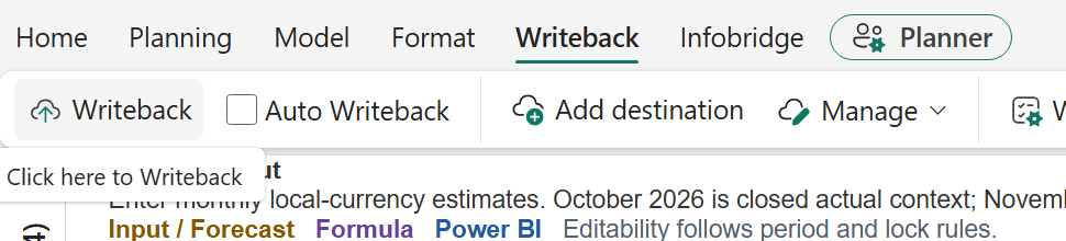
Open the Plan’s Writeback tab and select Add destination.

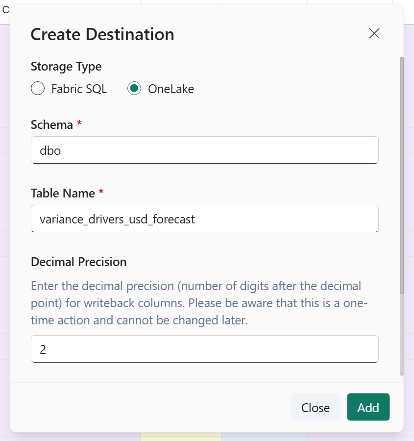
In Create Destination, select OneLake. Enter the Schema, Table Name, and Decimal Precision, then select Add.
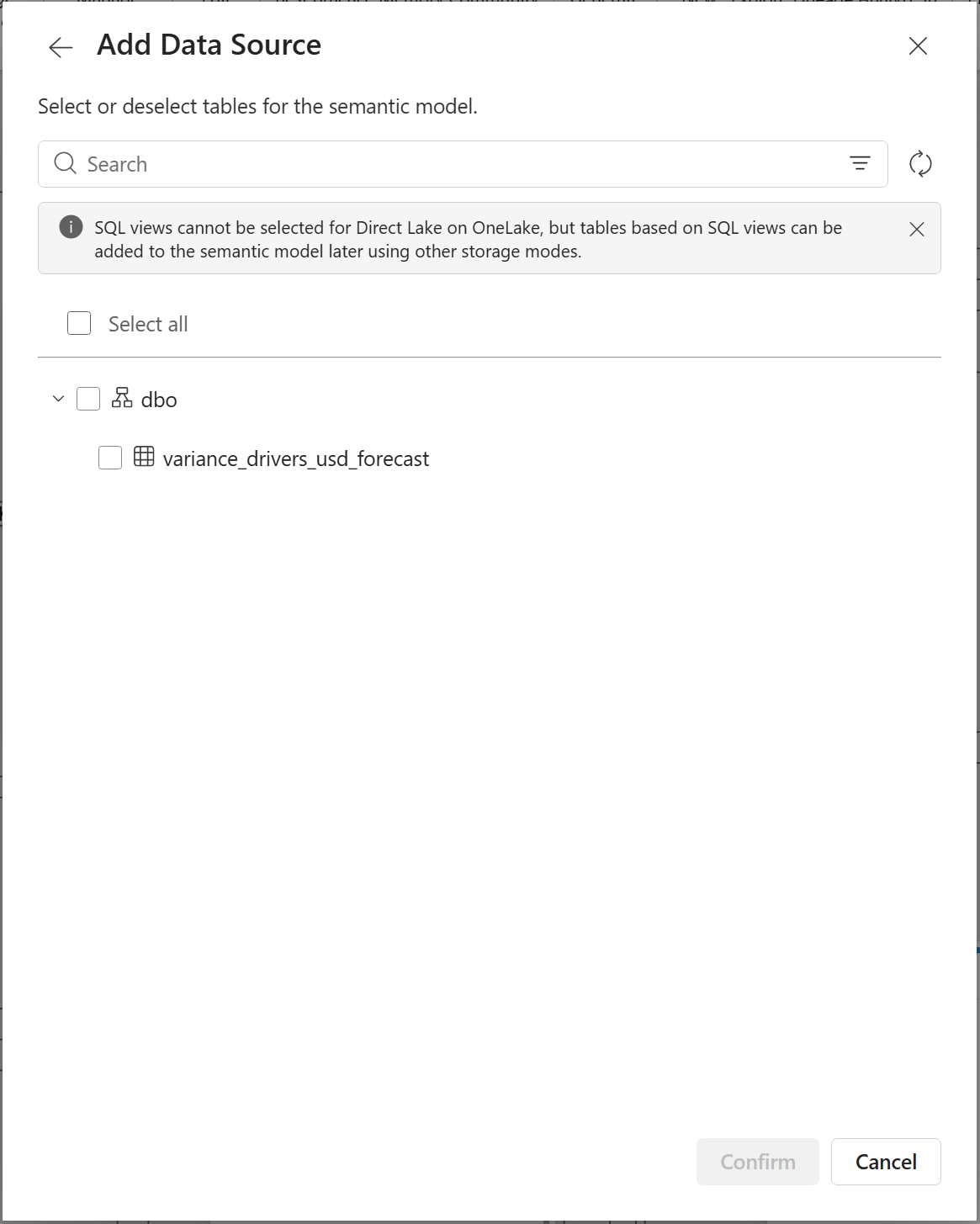
The example uses dbo, variance_drivers_usd_forecast, and two decimal places. The dialog notes that decimal precision cannot be changed later.
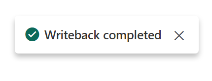
Select Writeback. When the operation finishes, the Plan displays Writeback completed.
Open Logs and confirm Destination Type: OneLake and Status: Success.

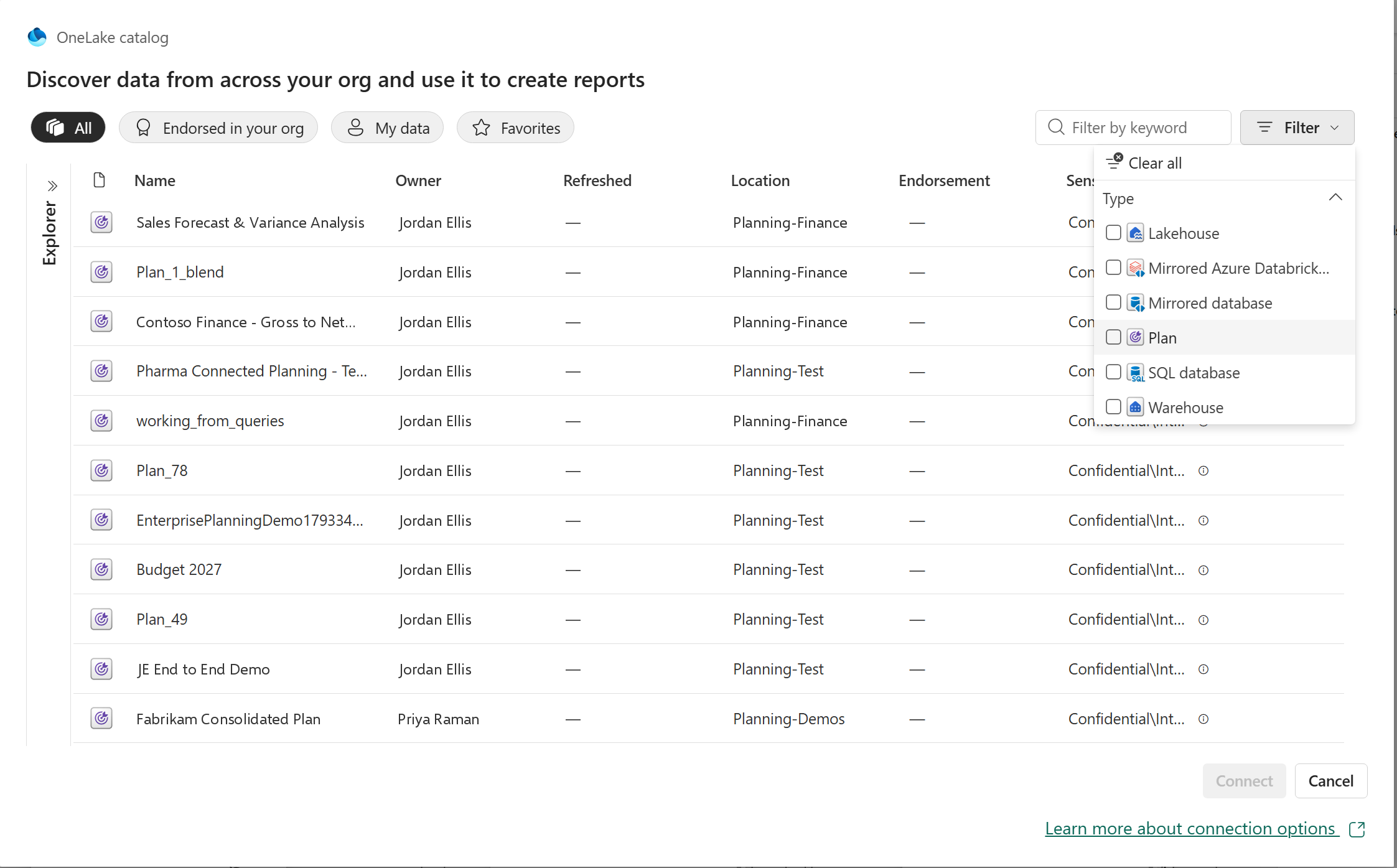
Plan items are now a supported source in the OneLake catalog. Each Plan item can contain multiple writeback tables; choose the ones your semantic model needs.
In the semantic model editor, select OneLake catalog. Open the top-right Filter, choose Type → Plan, select the Plan item, and select Connect.
The Add Data Source dialog lists the available writeback tables in the selected Plan. Expand the schema, select one or more tables, and select Confirm.
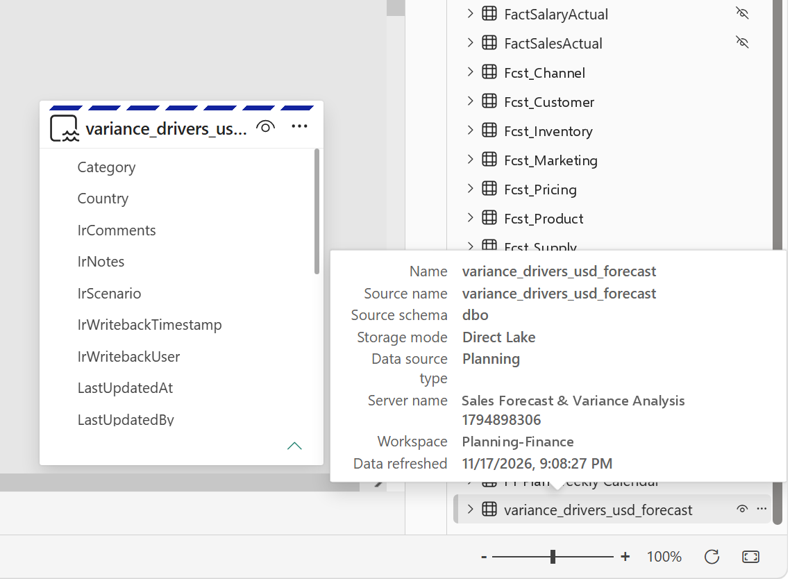
The selected table is added to the semantic model in Direct Lake mode. Hover over the table to inspect its details: Storage mode shows Direct Lake, and Data source type shows Planning.
Create a shortcut in the lakehouse’s Tables area that points to the Plan’s Delta table in OneLake. The lakehouse can use the table without another copy of the output. About OneLake shortcuts
With the writeback table available through the lakehouse, bind it to the relevant entity types and properties in Fabric ontology. This brings planning outputs into the business relationships used by that ontology. Ontology data binding
The reuse path: OneLake writeback table → Lakehouse shortcut → Ontology.
To start pipelines, refreshes or alerts automatically after each writeback, see Writeback that sets work in motion.
The screenshots show the writeback and semantic-model workflow; observed run times are examples, not performance guarantees.
A brand new in-memory engine for planning in Microsoft Fabric, with 10x+ improvements in both performance and scale. No separate system database is required anymore.
This is Part 1 of our three-part Native Planning Engine series. Part 2 covers writeback to OneLake, and Part 3 covers the performance improvements across Fabric Plan.

The scale figure compares the Native Planning Engine’s 12M-cell aggregate limit with 1.2M cells on the previous planning engine. The calculation figure is compared with the March preview; for writeback, the full benchmark in Part 2 shows up to 13× at 12M cells. Performance varies with semantic model design and capacity. For every user-facing improvement, see Part 3.
You can now enable the Native Planning Engine in Tenant settings as a Public Preview capability, as announced on our roadmap at FabCon Barcelona. Planning inputs are stored in OneLake as Apache Arrow files and loaded in memory for planning, so Plan items no longer need a separate system database.
We are also excited to share that you can now write back directly to OneLake as a new writeback destination, in Delta Parquet format. We cover that in Part 2: Writeback to OneLake.
In this article:
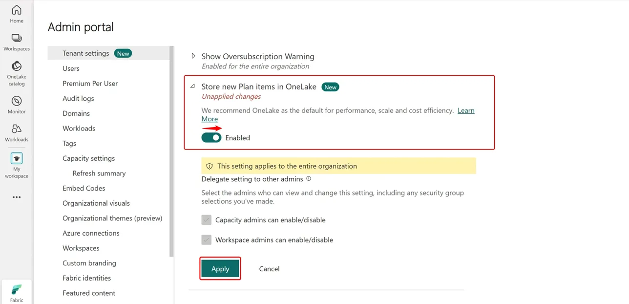
The Native Planning Engine is turned on by the Store new Plan items in OneLake setting. Once it is on, planning inputs are persisted in OneLake, and business output tables can write directly to OneLake as Delta Parquet. Turn the setting on at two levels.
Your Fabric administrator opens the Admin portal, goes to Tenant settings, turns on Store new Plan items in OneLake, and selects Apply.
In the workspace that holds your Plan items, open Workspace settings, go to Plan settings under Delegated Settings, and turn on Store new Plan items in OneLake.
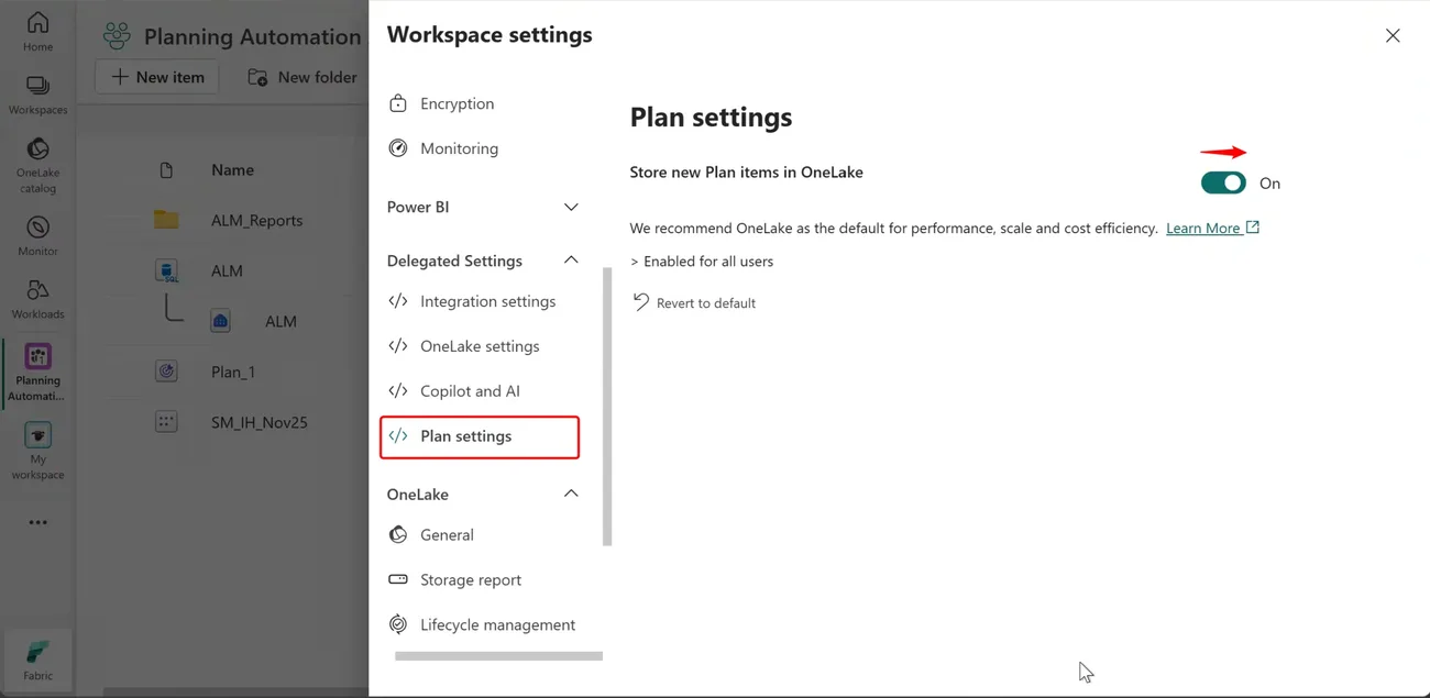
At general availability, every remaining Plan item moves automatically. GA is planned in the next few weeks. Plan items still on the previous planning engine will be migrated to the Native Planning Engine, so we recommend moving and checking your key items during the preview.
Fabric Plan now runs on a brand new native, file-based, in-memory planning engine that raises the planning limit tenfold, from 1.2 million to 12 million cells in aggregate. Apache Arrow supports efficient planning data access, while Delta Parquet makes business writeback outputs available across Fabric.
Plan items no longer need their own system database. Planning inputs live in OneLake, so there’s one less item to provision and manage, and storage is billed as part of your Fabric capacity. Fabric SQL remains a fully supported writeback destination, and PowerTable uses it as its writeback database.
Power BI semantic models can be massive, from millions to billions of rows or more. Because Fabric Plan runs directly on top of those semantic models, it can support any number of dimensions, measures and scenarios. That sets it apart from other planning tools, where performance degrades as the number of dimensions, measures or scenarios grows.
Any planning method, with the controls to run it across every line of business.
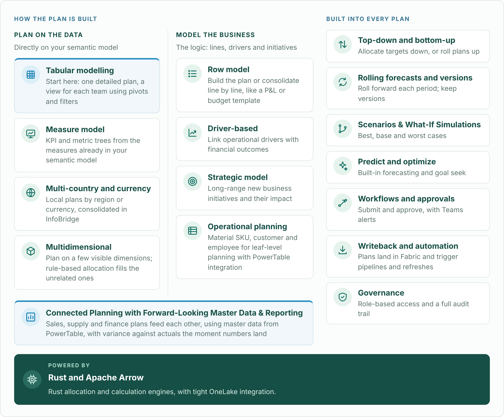
Go deeper: tabular modelling and choosing a planning method, measure models, row models, driver-based planning, operational planning with PowerTable, writeback and automation, and governance with Audit Cell History.
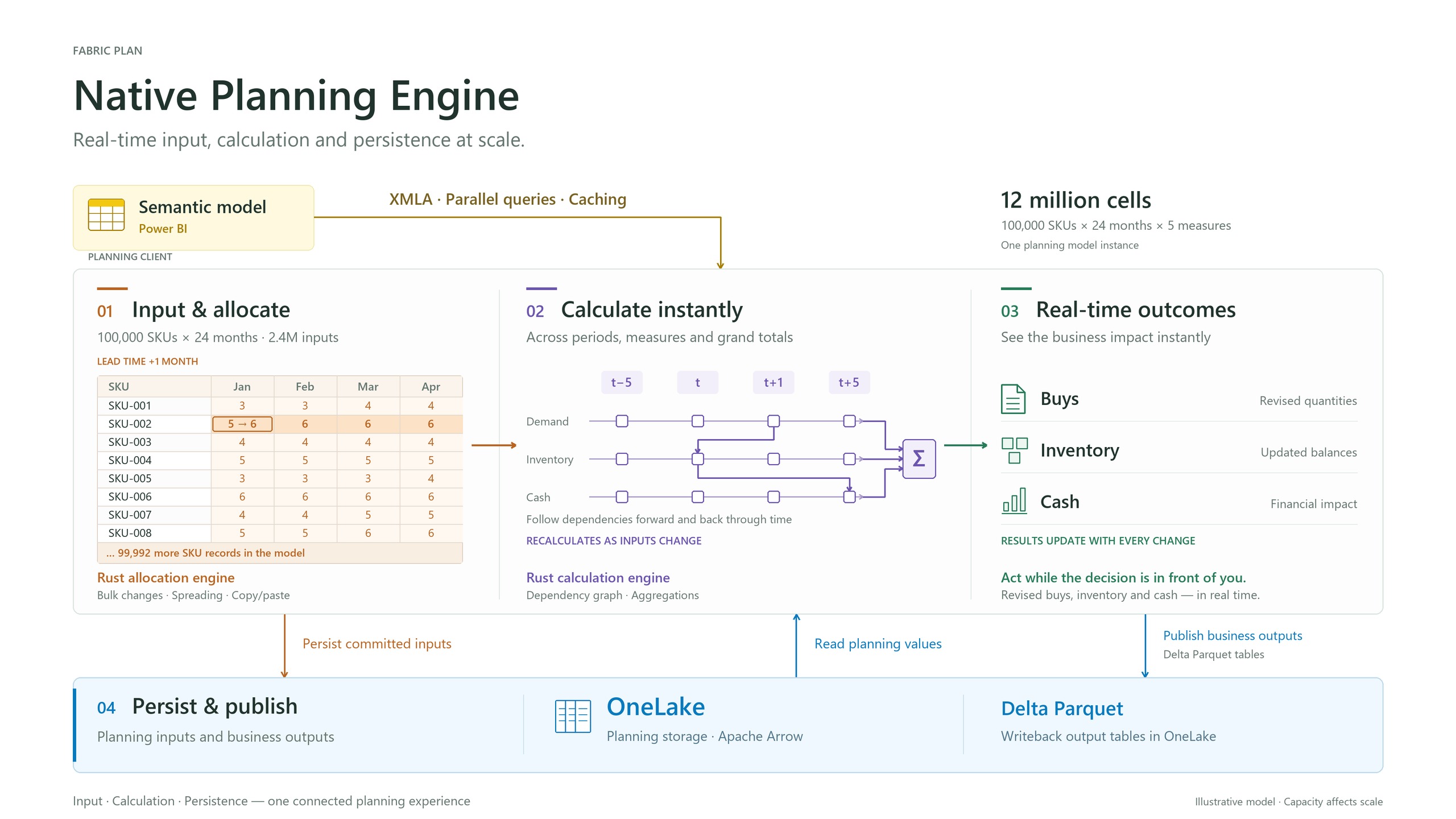
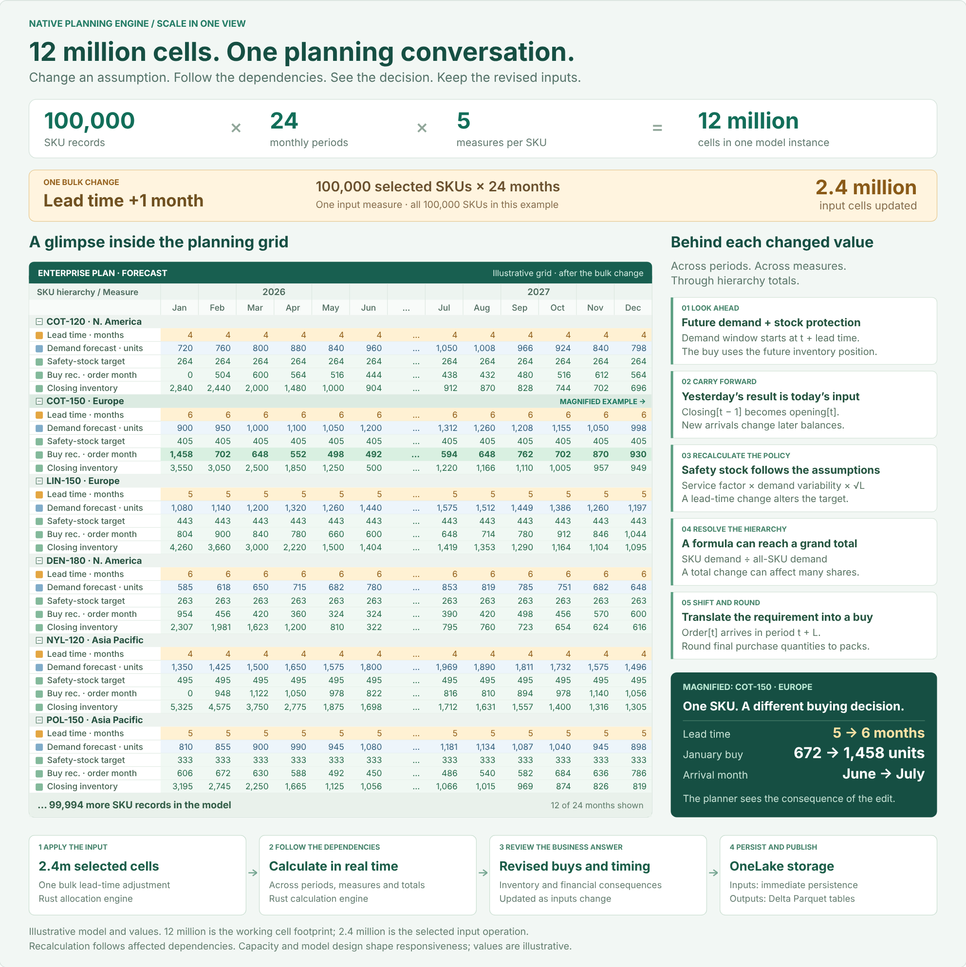
The illustration shows 12 million model cells, with 2.4 million cells affected by the bulk input operation.
Data fetched through XMLA affects capacity and responsiveness. The size of an interactive planning model is distinct from the volume published in a writeback instance. For scaling techniques such as context filtering, dimension partitioning, cubes and PowerTable, see Key Considerations for Planning at Scale with Microsoft Fabric Plan.
Caution: watch your Power BI XMLA query and concurrency limits. Large plans can reach the XMLA query and concurrency limits of your Fabric capacity, which can cause throttling. Limits depend on your capacity size, so consider a larger capacity when you need to fetch more Actuals data per query from the semantic model.
With this release, the Native Planning Engine supports up to 12 million cells in aggregate, 10x the 1.2 million cells of the previous engine. That total covers Actuals fetched from your semantic model plus visual forecast and formula measures. Next on our roadmap is support for up to 120 million cells inside the planning grid, 100x the previous limit. At that point, the only limit will be how much data you can fetch efficiently from your semantic models without throttling. Data fetched through XMLA alone will be capped at around 12 to 24 million cells.
This is a forward-looking roadmap item; release timing may change.
The Native Planning Engine is our default recommendation going forward.
Advanced modeling features require OneLake storage. Audit cell history and driver-based modeling are available now, and snapshots (frozen versions) arrive on December 8, 2026. These capabilities are supported only by the Native Planning Engine: they require its file-based architecture and will not be supported by the previous planning engine.
Fabric SQL remains a fully supported writeback destination.
A Fabric administrator turns on Store new Plan items in OneLake in Tenant settings. The setting can be delegated so that capacity and workspace admins can enable or disable it, and it is then turned on for each workspace in Workspace settings → Plan settings. See Turn on the Native Planning Engine.
No. The setting applies to new Plan items. Existing items keep running on the previous planning engine until you migrate them, or until the automatic migration at general availability.
Yes, but not as the system database. Planning inputs are now stored in OneLake, which removes the need for a second database. PowerTable continues to use Fabric SQL as its writeback database, and Planning sheets continue to support Fabric SQL as a writeback destination, alongside OneLake writeback.
Migrating an item from Item settings moves that item to the new engine. Copying an item with deployment pipelines creates a new item without its data, which is useful for testing. The recommended path is to smoke test first: copy the item with deployment pipelines, check it on the Native Planning Engine, then migrate the original from Item settings.
No. Migration is one-way, so a migrated item can’t be moved back to the previous planning engine. Smoke test a copy first, as described above, before migrating the original.
Once every Plan item in the workspace has been migrated to OneLake, the Fabric SQL system database (the application database) can be safely deleted. If any Plan items in the workspace haven’t been migrated yet, leave the database in place so their metadata isn’t lost. Keeping it does no harm.
The pricing model doesn’t change: Fabric Plan is still billed by session type on your Fabric capacity. What changes is the other resources part of the bill. Instead of charges for a Fabric SQL system database, you now incur OneLake storage. See how Fabric Plan pricing works.
No. There are no known limitations during the preview.
The inventory illustration uses fictional data. Performance figures are examples, not performance guarantees.
Audit Cell History in Fabric Plan shows who changed a planning cell, what changed, and when, and lets you undo any user’s change by restoring an earlier value. It is available now with the Native Planning Engine, in Public Preview.
Return any selected cell to a value recorded by any user at any point in its available history.
Choose an entry from the cell’s timeline and restore that exact value. The restoration is captured as a new auditable change, so recovery does not break the history.
Important compatibility note: Cell History is available only with the Native Planning Engine. It relies on the engine’s file-based architecture in OneLake and is not supported by the previous planning engine.
Fabric Plan already provides a detailed audit experience. The Data Input tab captures sheet-wide data activity: tag, action, row, column, old value, new value, user, and timestamp. The Reports tab captures report changes such as scaling, columns, and formatting.
Cell History complements those broad views with a focused, actionable timeline for the value a planner has selected. The row, measure, period, user, action, and value transitions are presented together, directly beside the planning grid. A planner can then select any recorded entry and restore that exact value to the cell.
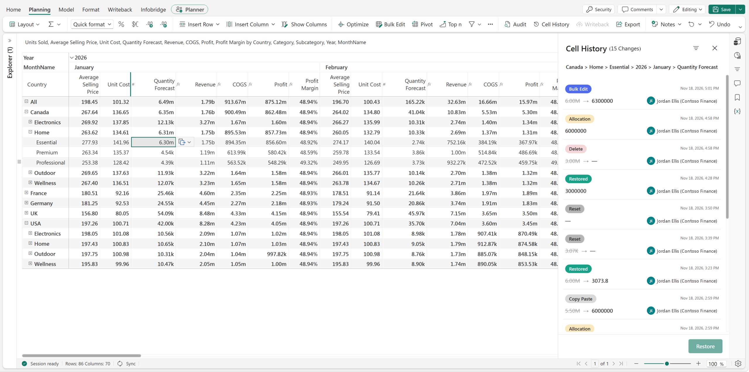
Select the January Quantity Forecast for Canada › Home › Essential (6.30M) and open its complete change story in context.
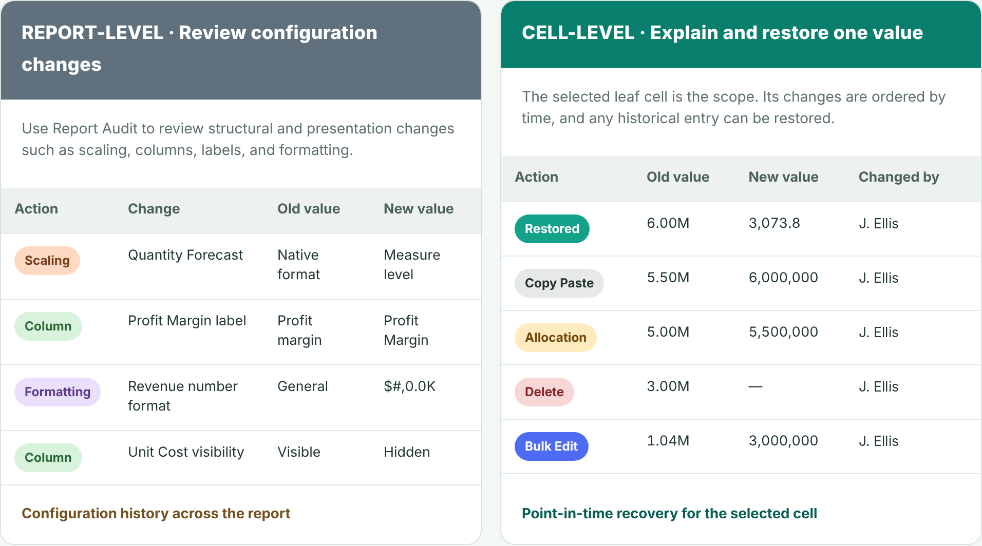
Report Audit explains how the report changed. Cell History explains, and can restore, one planning value.
Cell History is available for a leaf-level data-input cell. Select a specific intersection of business context and time, such as Canada, Home, Essential, January 2026, Quantity Forecast, and open Cell History. The side panel keeps that complete coordinate visible while it lists the recorded changes from newest to oldest.
Canada › Home › Essential › 2026 › January › Quantity Forecast
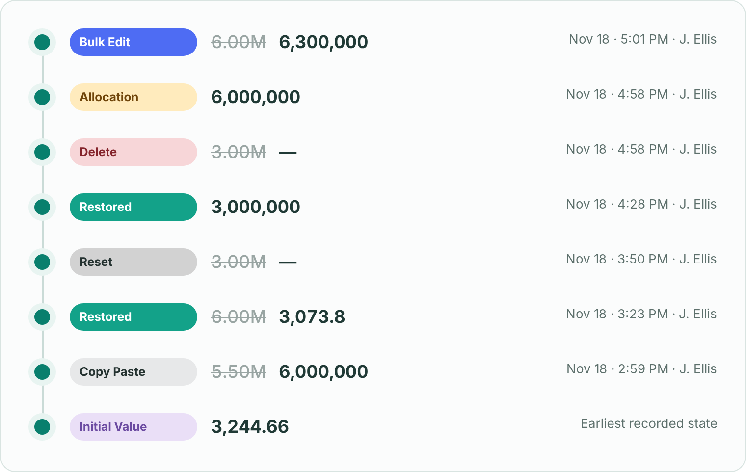
Each entry identifies the mechanism that produced the change. A leaf value may have changed through direct input, an allocation from a parent, a bulk update, or pasted values. Cell History keeps those actions distinct.
| Change type | What it means |
|---|---|
| Initial Value | The earliest recorded state of the cell, before any tracked change. |
| Allocation | A value entered at a parent or subtotal was distributed down to this leaf cell. |
| Manual Input | A planner directly edited this leaf-level value in the grid. |
| Bulk Edit | The cell changed as part of a multi-cell update configured through Bulk Edit. |
| Copy Paste | The value was pasted from another grid range or from outside the planning experience. |
| Delete | The planned value was removed, leaving the leaf cell blank until another action supplied a value. |
| Restored | A user intentionally returned the cell to one of its recorded historical values. |
| Reset | The cell returned to its configured default, or to blank when no default exists. |
A cell can accumulate many changes. The filter panel narrows the list while the selected cell remains fixed.
Show only allocations made by a specific user, isolate deleted values or manual inputs, or limit the list to a selected date range.
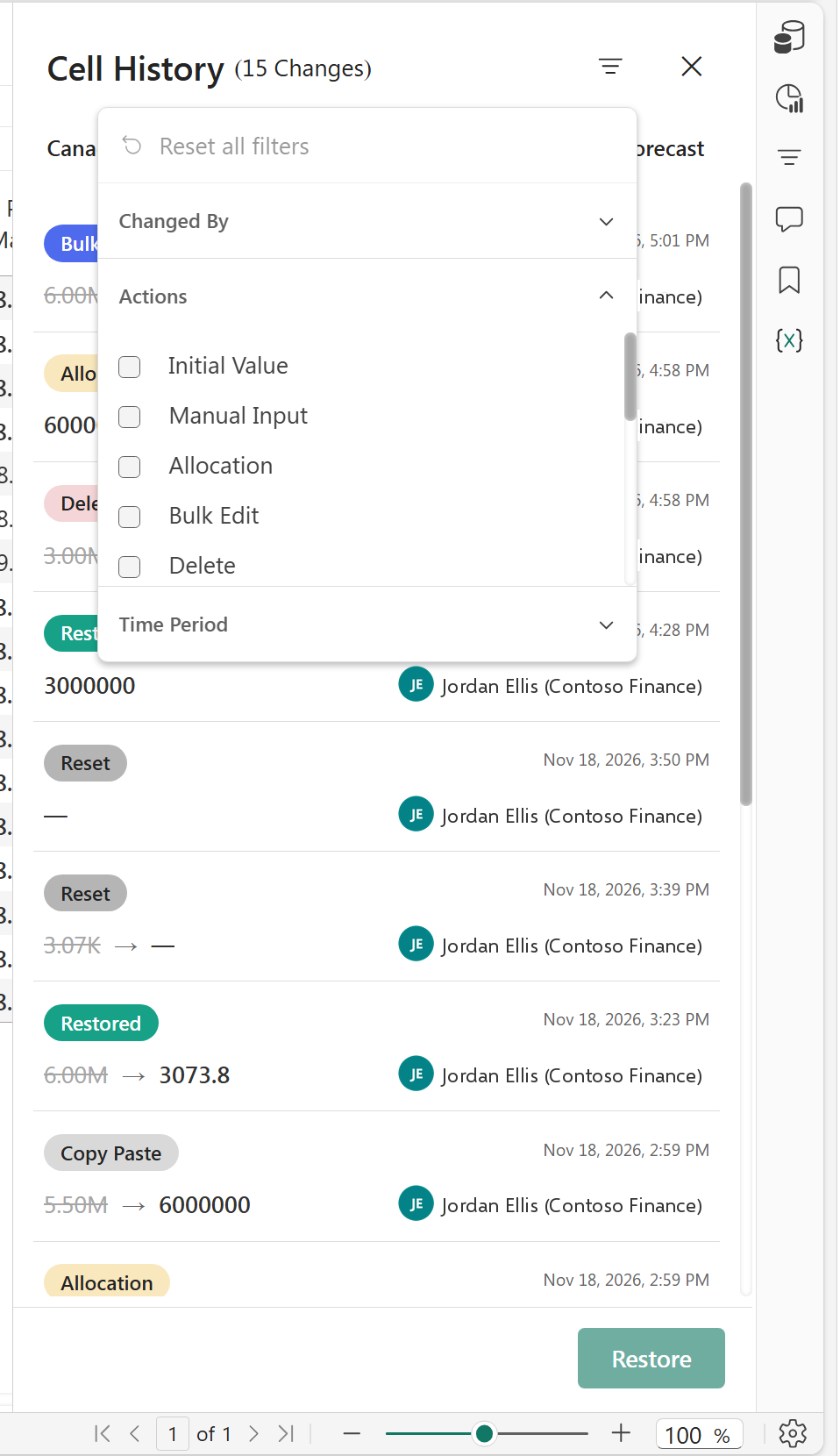
Use Changed By, Actions, or Time Period to locate the exact entry. Select it and choose Restore to return the leaf cell to that recorded value, regardless of which user originally made the change. The restoration is recorded as another change in the cell history.
| Action | What it does |
|---|---|
| Restore | Return the selected cell to a specific value from any point in its available history. |
| Delete | Remove the current planned value. Cell History records the old value changing to blank as a Delete action. |
| Reset | Remove the current planned input and return the cell to its configured default. If the default is blank, the cell returns to blank. |
The two experiences are complementary. Audit is designed for broad review and export, while Cell History is designed for focused investigation and recovery at the selected leaf-level cell.
| Capability | Audit | Cell History |
|---|---|---|
| Scope | Entire report history across data-input and report-configuration activity | One selected leaf-level cell |
| Change context | Report-wide records for review and governance | Who changed it, What changed, and When |
| Undo and Restore | Not supported | Undo a specific change by restoring its selected historical value |
| Export | Export the entire report history to Excel | Cell-level history export is not supported |
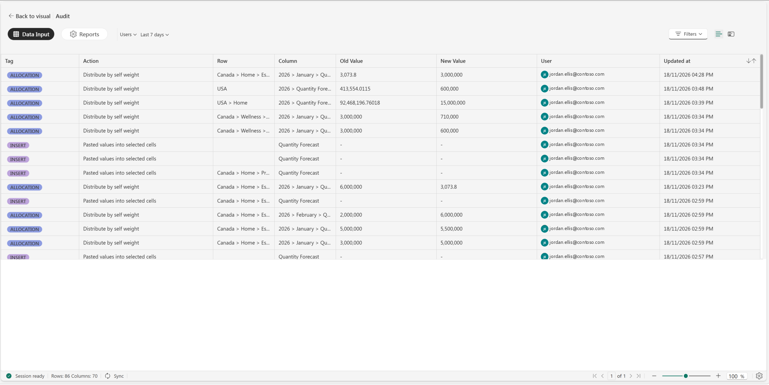
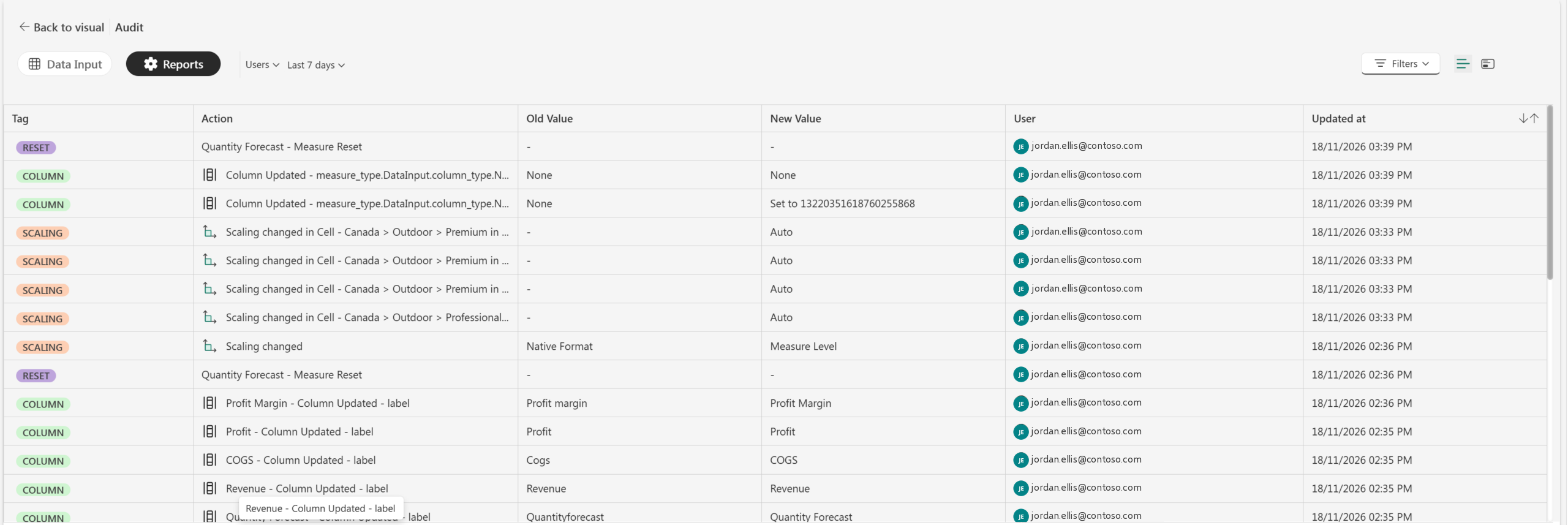
Cell History turns audit information into a recovery workflow. A planner can see whether a value came from a direct edit, allocation, bulk update, paste, or deletion; identify the user and time; and restore the exact recorded value from any selected point in the cell’s available history.
The feature is intentionally narrow: it applies to a selected leaf-level input cell. Sheet-wide data changes remain in Data Input audit, and report configuration changes remain in Reports audit.
Feature details reflect Fabric Plan at the time of writing.
Open a Plan app that several teams share and Explorer lists every sheet you have access to. For the person who built the app, that’s fine. For a sales manager who opens it twice a month, it’s a long list with no obvious place to start. And someone who wears two hats, say sales and HR, gets both lists mixed together.
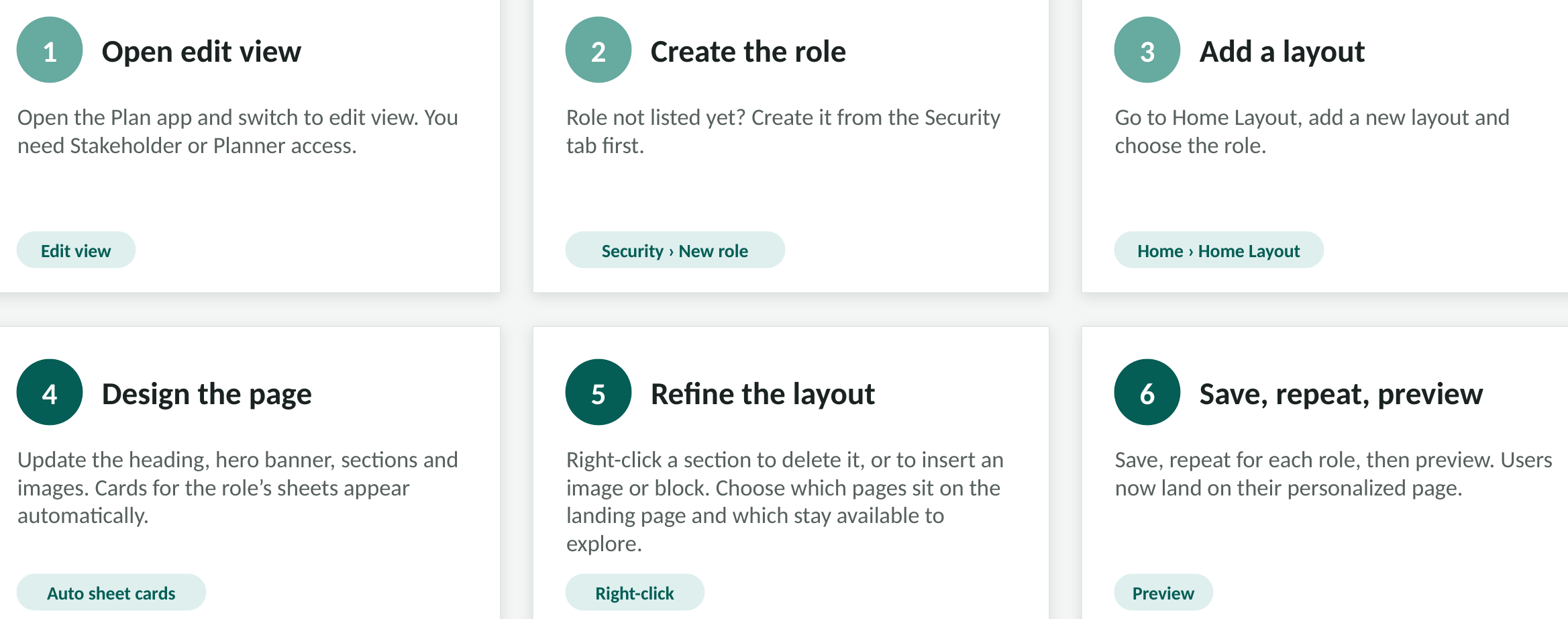
Home Layout gives each security role its own landing page with its own sheets, so sales lands on a sales page and HR on an HR page in the same app.

Here’s one built for a sales manager. The numbers match the callouts below.
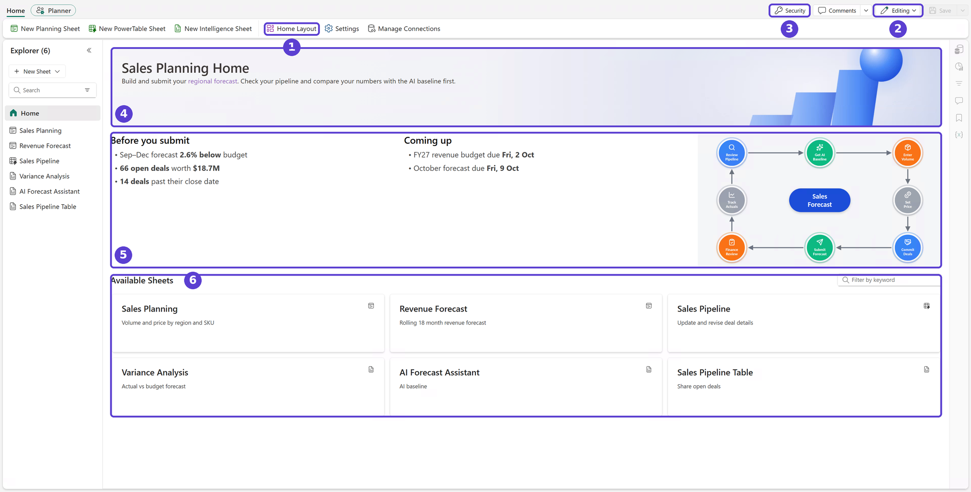
Each role sees the sheets meant for it. When finance, sales and HR share one Plan app, that helps keep unauthorized views out of reach and supports segregation of duties. People also spend less time wading through modules they don’t use.
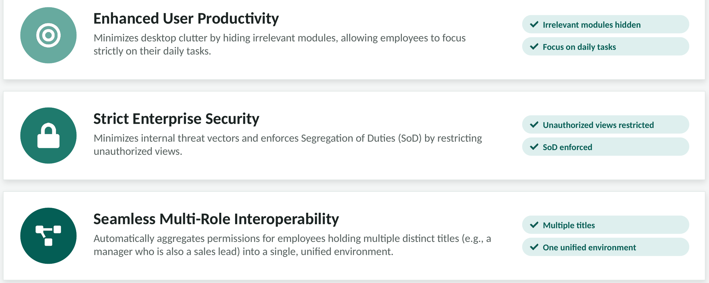
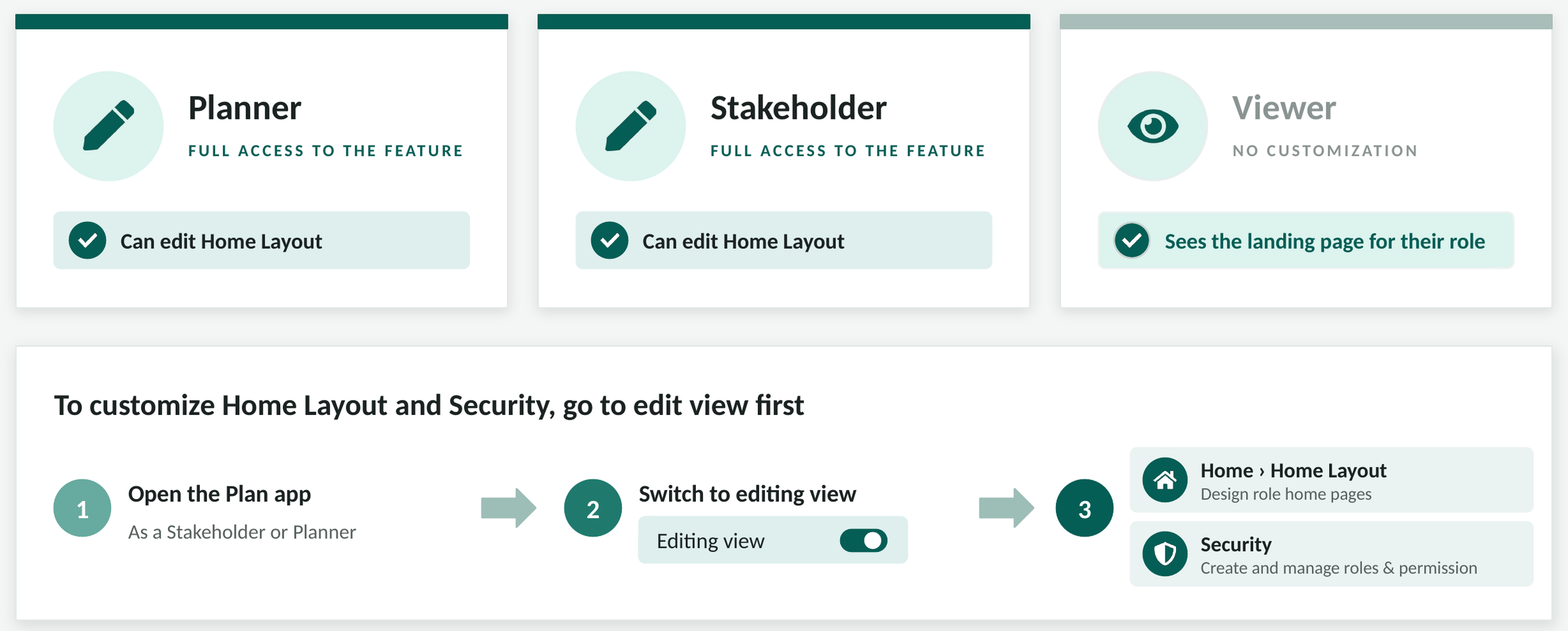
Anyone in a Stakeholder or Planner session can edit Home Layout. Viewers can’t change it; they see the page for their role. Admins decide who can open Stakeholder or Planner sessions in the first place, so page design stays with the people you’ve picked.
To change Home Layout or Security, switch to editing view first. Home Layout is on the Home tab and Security is at the top right.
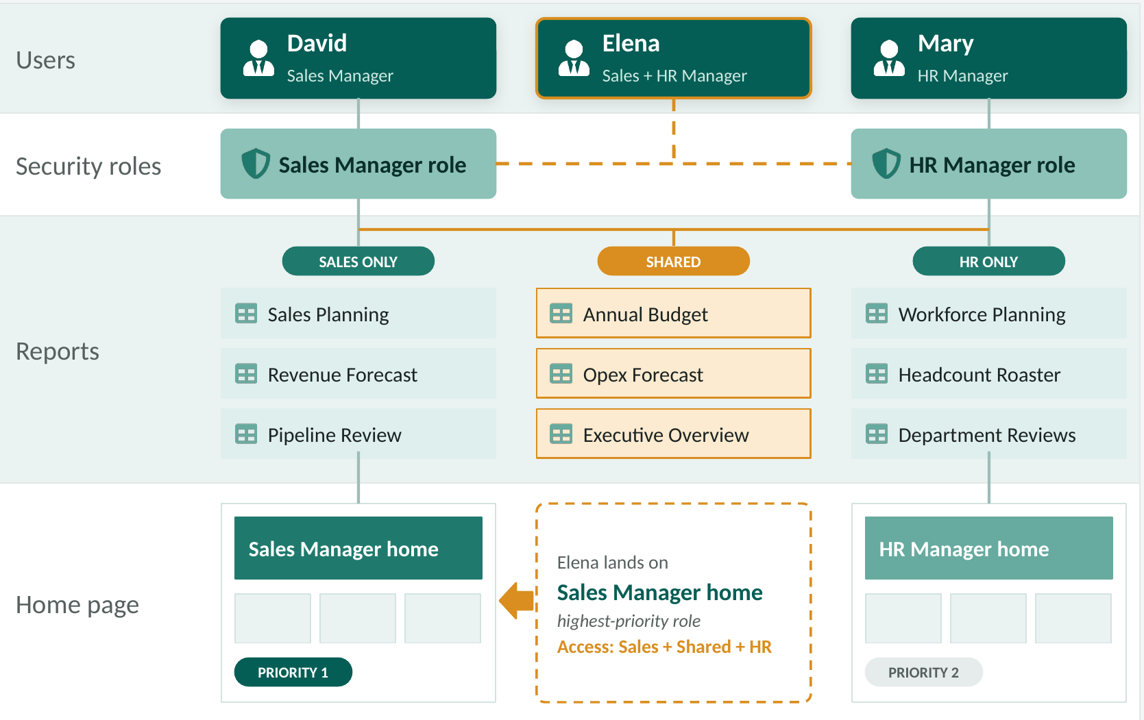
Real org charts aren’t tidy. David is a sales manager and Mary runs HR. Elena does both, so she holds both roles. Her access is the sum of the two: the sales sheets, the HR sheets and the ones they share. Her landing page comes from her highest-priority role, here the Sales Manager home. Give the higher priority to the role people work in every day.
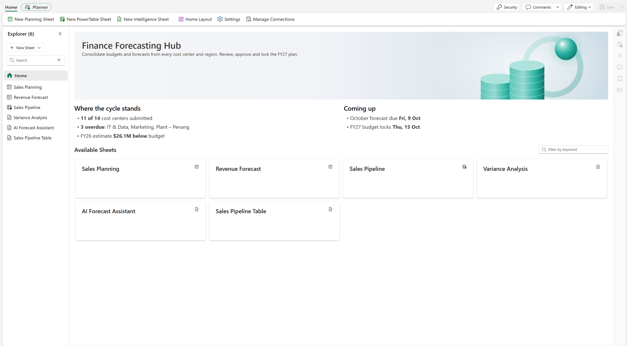
Finance uses its page to say where the cycle stands: how many cost centers have submitted, which are overdue and when the budget locks.
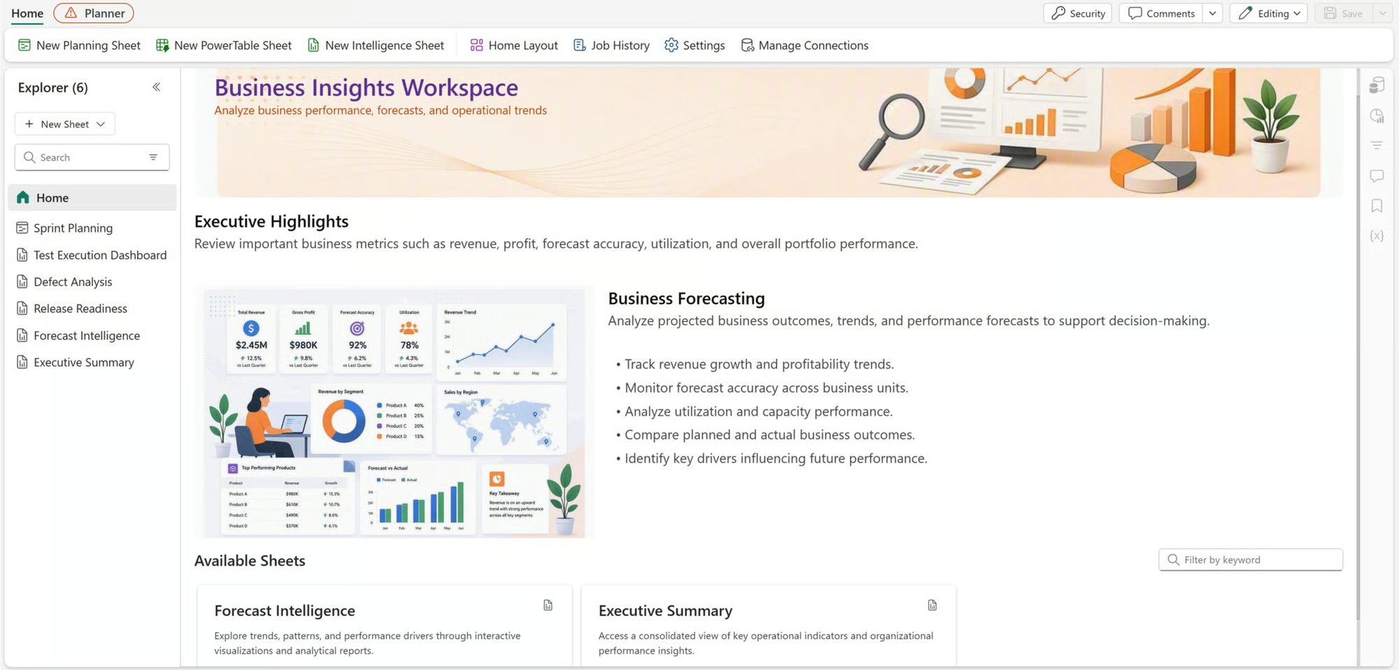
An executive page leads with highlights and a short read on the forecast before anyone opens a sheet.
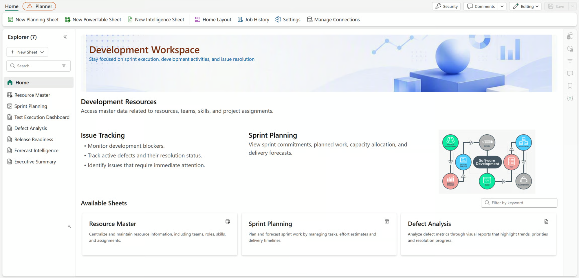
Home Layout isn’t only for finance. This development team’s page leads with issue tracking and sprint planning.
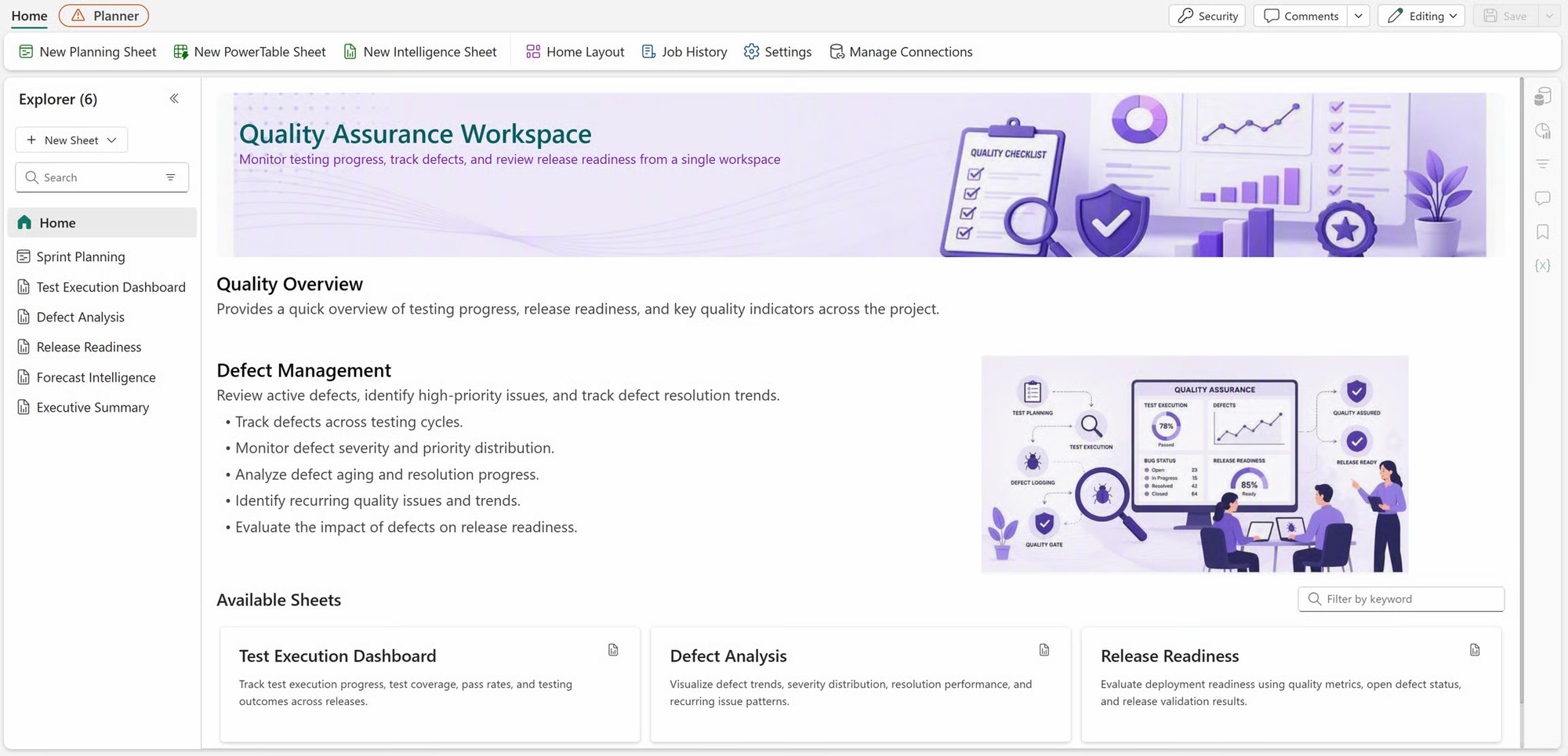
Quality assurance gets its own view of the same release work: testing progress, defects and release readiness.
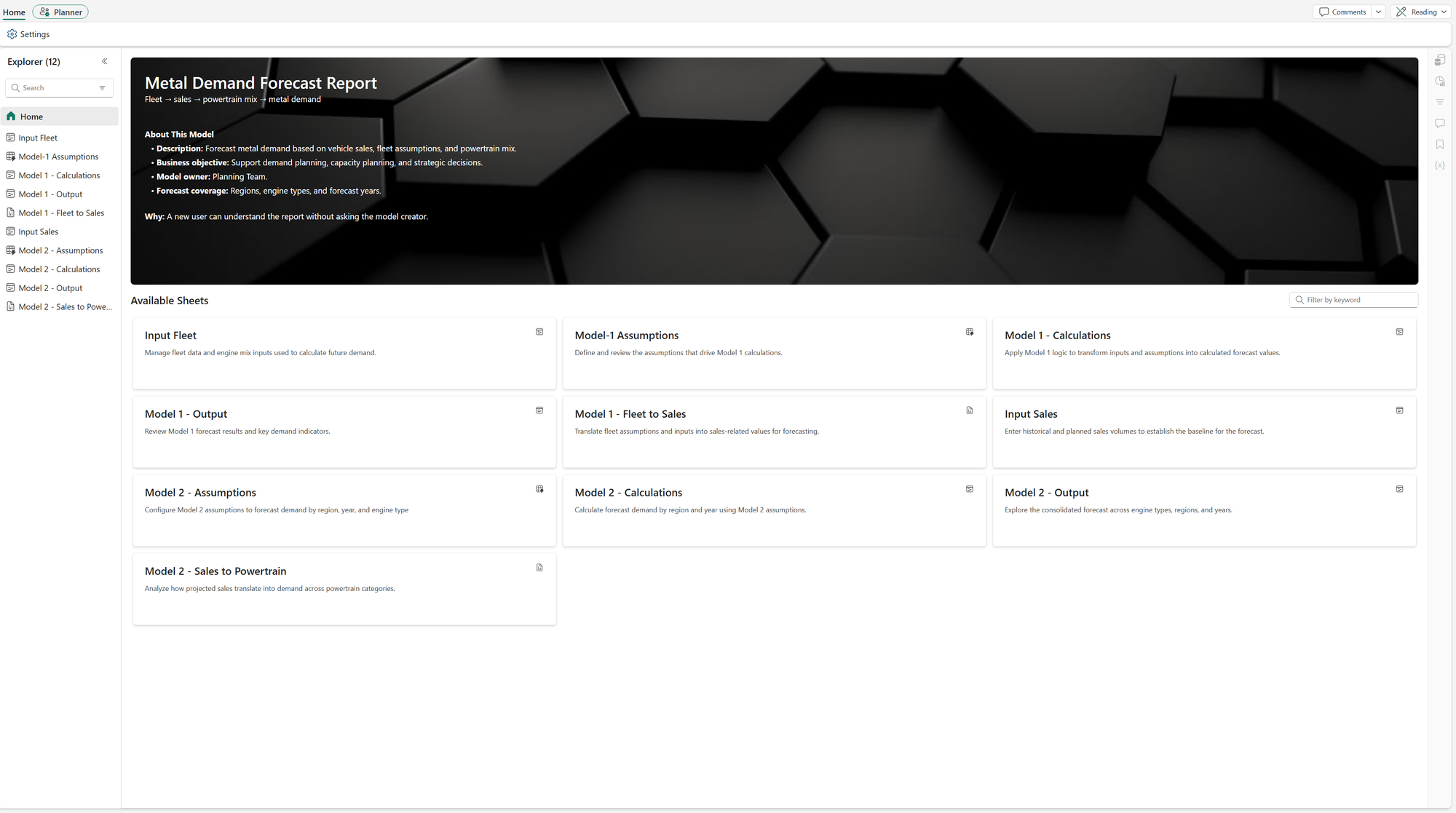
A home page also works as documentation. A new user reads what the model does and who owns it before opening a single sheet.
Home Layout follows your security roles, so set up the roles and their sheet access in Security before you design any pages. A tidy role setup makes the pages quick to build. Then preview every role before you tell people it’s live.
One of the first decisions when you build a plan in Fabric Plan is to choose between Row Model or Measure Model. They both have capabilities that are common. For example, both can give you a P&L plan that expands and collapses. Underneath, they’re built differently. That affects what you maintain day to day and how much work it takes when you add a product or a forecast version later.
In a Row Model (earlier known as model builder) you build the business hierarchy yourself, row by row. In this example, you have the GL lines in a hierarchy that helps you calculate gross profit and net profit. The measures carry the series, such as Actuals, Budget and Forecast.
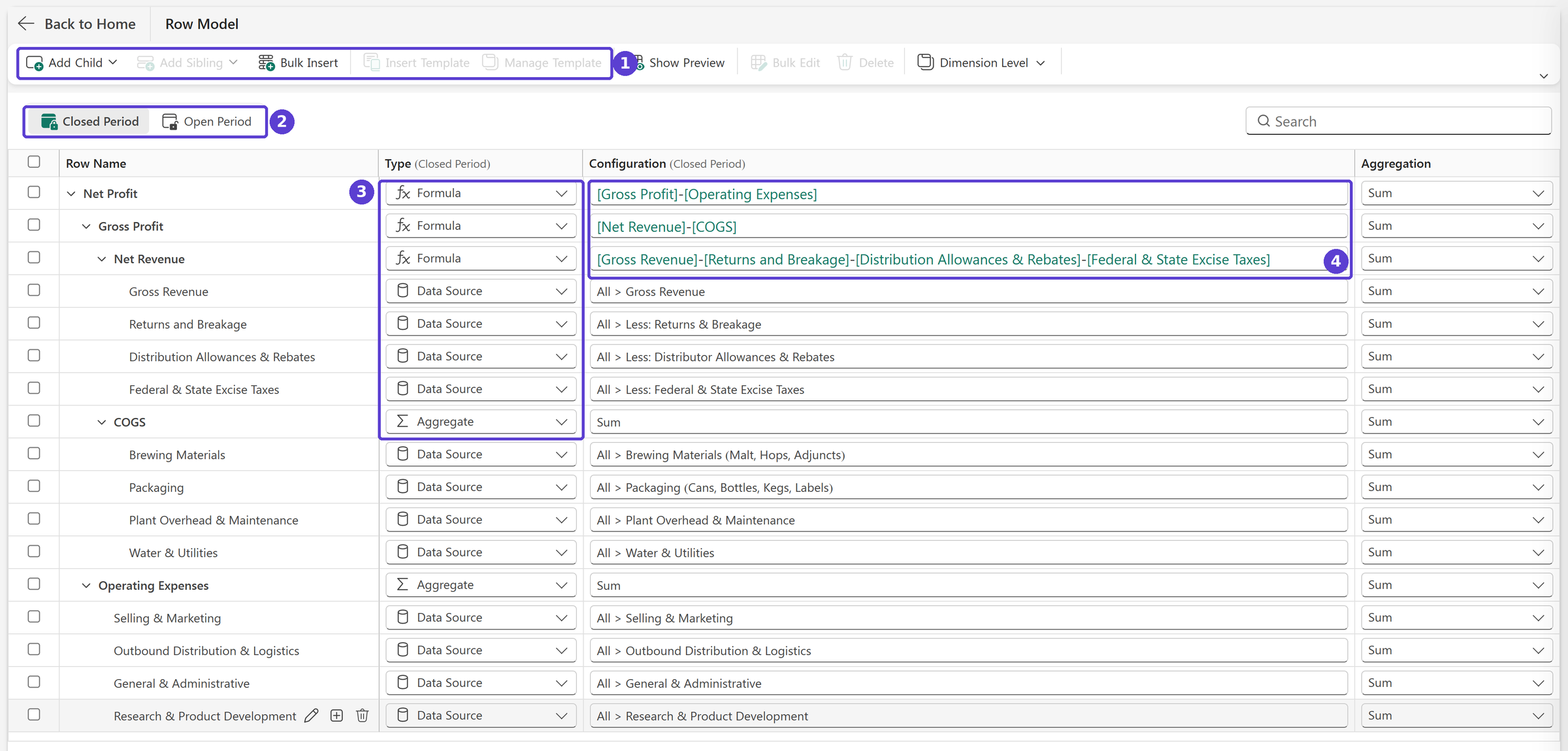
Every row has its own logic, but they use a common measure (e.g., actuals, plan, forecast).
This is how the app looks once you have built out the row model.
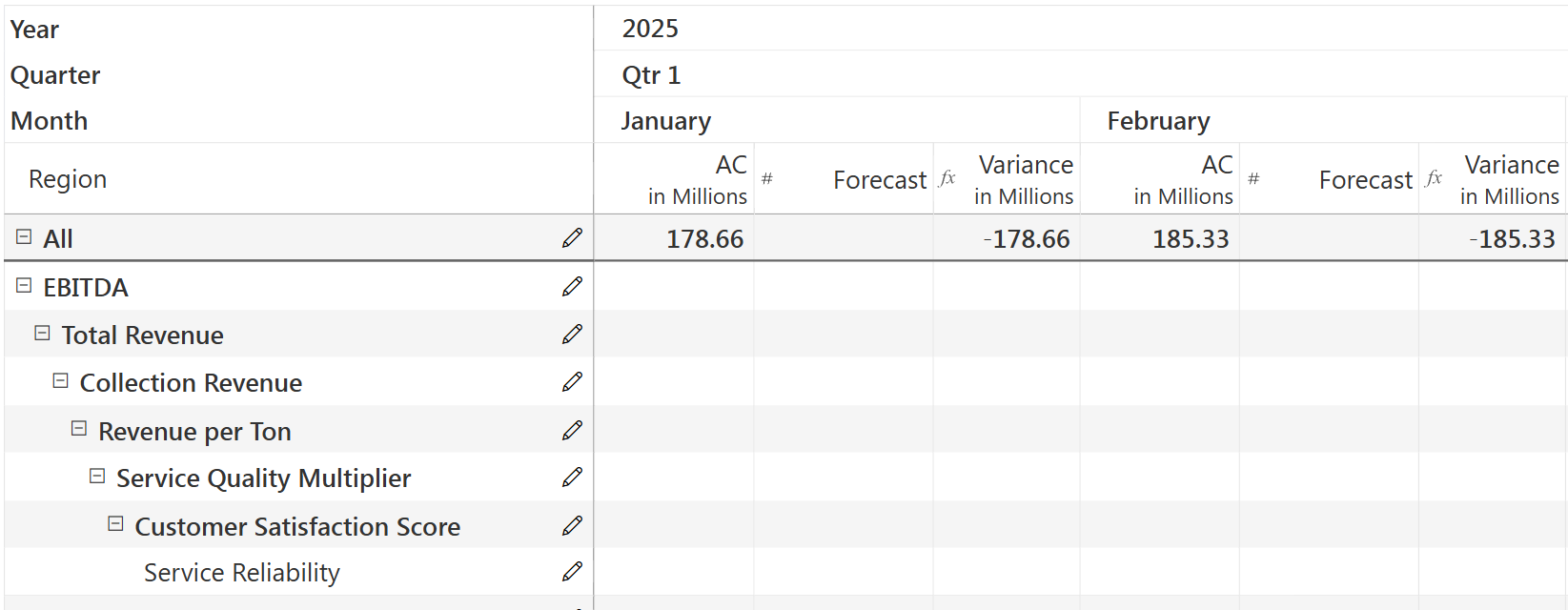
If you need a second forecast, add a Forecast V2 measure. It reuses the same business hierarchy in the rows.
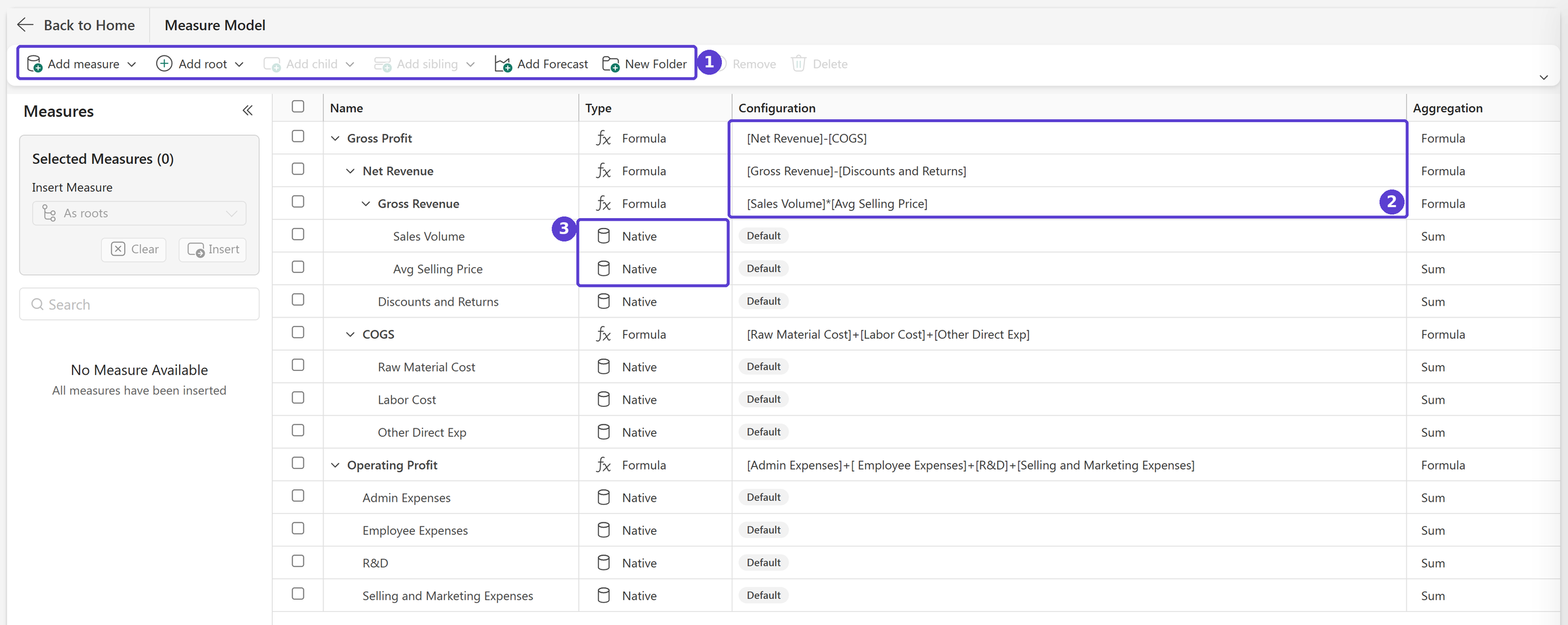
In a Measure Model the KPIs are measures. Many of them already exist in your semantic model as DAX measures, and you build on top of them.
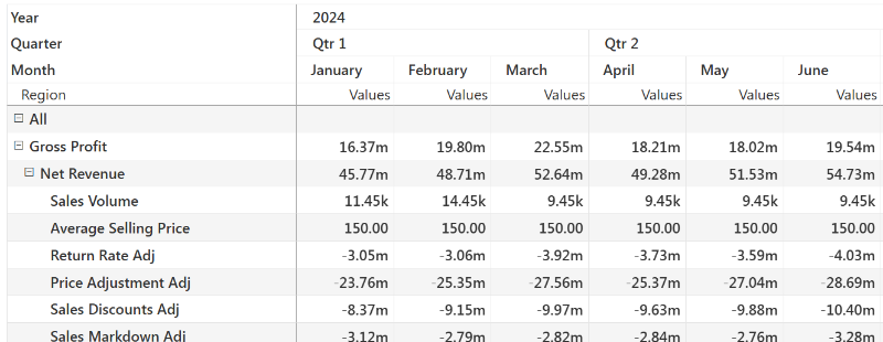
When you display the measures in rows, it looks very similar to a Row Model. When you check the column header though, It will say ‘Values’. Unlike the row model, each row here is a measure.
Look down one column. If every row follows the same formula, go with Measure Model. Sales is a typical usual case: Revenue = Units × Price for every product.
If the logic changes from row to row, with some rows as inputs and others as formulas, go with Row Model. A P&L works that way.
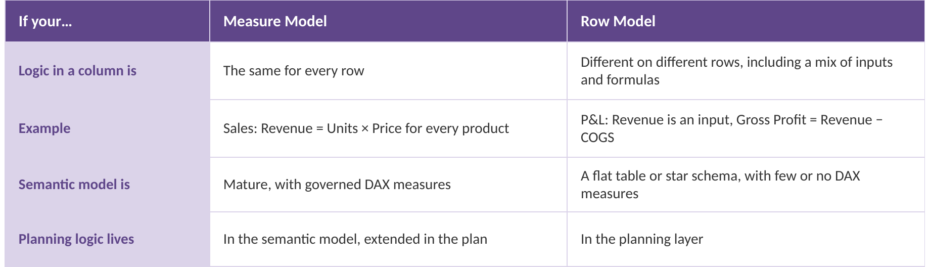
The semantic model is a tiebreaker. If you already have governed DAX measures, Measure Model reuses them. If you’re working off a flat table or a star schema with few measures, Row Model puts the logic in the plan.
The planning work itself points the same way. Comparing Actuals, Budget and several forecasts on one KPI hierarchy is easier in Row Model. A focused forecast built from KPI relationships fits Measure Model better.
Drivers shouldn’t sway this choice. Driver-Based Planning isn’t a third model. It sets an input to follow another value, like marketing at 6% of revenue. It works the same way on Row Model and Measure Model sheets. Here’s one January plan with $2M revenue and $120k marketing, shown in each.
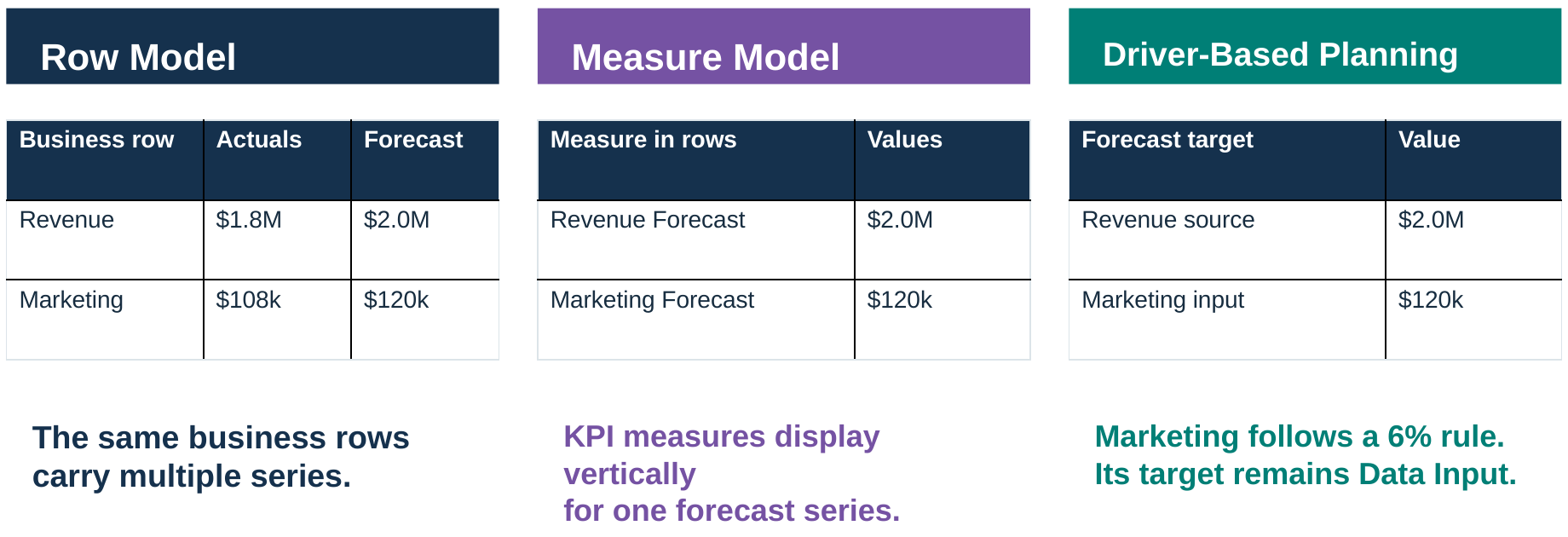
So pick the structure first based on the nature of your dimensions and measures. Then go for a model that suits you best.